NOAA Teacher at Sea Dieuwertje “DJ” Kast Aboard NOAA Ship Henry B. Bigelow May 19 – June 3, 2015
Mission: Ecosystem Monitoring Survey
Geographical area of cruise: East Coast Date: May 25, 2015, Day 7 of Voyage
Interview with Emily Peacock
Emily Peacock and her ImagingFlowCytobot. Photo by: DJ Kast
Emily Peacock is a Research Assistant with Dr. Heidi Sosik at the Woods Hole Oceanographic Institution (WHOI). She is using imaging flow-cytometry to document the phytoplankton community structure along the NOAA Henry B. Bigelow Route.
Why is your research important?
Phytoplankton are very important to marine ecosystems and are at the bottom of the food chain. They uptake carbon dioxide (CO2) and through the process of photosynthesis make oxygen, much like the trees of the more well-known rain forests.
The purpose of our research is “to understand the processes controlling the seasonal variability of phytoplankton biomass over the inner shelf off the northeast coast of the United States. Coastal ocean ecosystems are highly productive and play important roles in the regional and global cycling of carbon and other elements but, especially for the inner shelf, the combination of physical and biological processes that regulate them are not well understood.” (WHOI 2015)
What tool do you use in your work you could not live without?
I am using an ImagingFlowCytobot (IFCB) to sample from the flow-through Scientific Seawater System.
ImagingFlowCytobot. Photo: DJ KastInside of the ImagingFlowCytobot. Photo by Taylor CrockfordThe green tube is what collects 5 ml into the ImagingFlowCytobot. Photo by: DJ Kast
IFCB is an imaging flow cytometer that collects 5 ml of seawater at a time and images the phytoplankton in the sample. IFCB images anywhere from 10,000 phytoplankon/sample in coastal waters to ~200 in less productive water. Emily is creating a sort of plankton database with all these images. They look fantastic, see below for sample images!
Microzooplankton called Ciliates. Photo Credit: IFCB, from this Henry Bigelow research cruise.Dinoflagellates Photo Credit: IFCB, from this Henry Bigelow research cruise.
The IFCB “is a system that uses a combination of video and flow cytometric technology to both capture images of organisms for identification and measure chlorophyll fluorescence associated with each image. Images can be automatically classified with software, while the measurements of chlorophyll fluorescence make it possible to more efficiently analyze phytoplankton cells by triggering on chlorophyll-containing particles.” (WHOI ICFB 2015).
What do you enjoy about your work?
I really enjoy looking at the phytoplankton images and identifying and looking for more unusual images that we don’t see as often. I particularly enjoy seeing plankton-plankton interactions and grazing of phytoplankton.
Grazing (all photo examples are not from this research cruise but still from an IFCB):
Small flagellates on a Thallasiosira (Diatom) Photo Credit: IFCB at MVCODiatom with a dinoflagellate eating it from the outside using a peduncle (feeding appendage). Photo Credit: IFCB at MVCOEngulfer- Gyrodinium will engulf the diatom Paralia Photo Credit: IFCB at MVCODinoflagellates pallium feeding externally, the pallium (cape-like structure, think of saran wrap on food) wraps around the prey. Photo Credit: IFCB at MVCO
What type of phytoplankton do you see?
I am seeing a lot of dinoflagellates in the water today (May 20th, 2015), Ceratium specifically.
Ceratium. Photo by IFCB at MVCO
The most common types of plankton I see are: diatoms, dinoflagellates, and microzooplankton like ciliates. The general size range for the phytoplankton I am looking at is 5-200 microns.
Colonial choanoflagellate. Photo Credit: IFCB at MVCO
Where do you do most of your work?
“The Martha’s Vineyard Coastal Observatory (MVCO) is a leading research and engineering facility operated by Woods Hole Oceanographic Institution. The observatory is located at South Beach, Massachusetts and there is a tower in the ocean a mile off the south shore of Martha’s Vineyard where it provides real time and archived coastal oceanographic and meteorological data for researchers, students and the general public.” (MVCO 2015).
Most of my work with Heidi is at the Martha’s Vineyard Coastal Observatory. IFCB at MVCO has sampled phytoplankton every 20 minutes since 2006 (nearly continuously). This unique data set with high temporal resolution allows for observations not possible with monthly or weekly phytoplankton sampling.
Below is an example from the MVCO from about an hour ago at 1 PM on May 20th, 2015.
Photo Credit: IFCB at MVCO
Did you know??
IFCB at Martha’s Vineyard Coastal Observatory has collected photos of nearby phytoplankton every 20 minutes since 2006 (9 years, almost continuously). With this time series, you can study changes in temporal and seasonal patterns in phytoplankton throughout the years.
NOAA Teacher at Sea Dieuwertje “DJ” Kast Aboard NOAA Ship Henry B. Bigelow May 19 – June 3, 2015
Mission: Ecosystem Monitoring Survey
Geographical area of cruise: East Coast Date: May 22, 2015, Day 4 of Voyage
Interview with Jessica Lueders-Dumont
Who are you as a scientist?
Jessica Lueders-Dumont is a graduate student at Princeton University and has two primary components of her PhD — nitrogen biogeochemistry and historical ecology of the Gulf of Maine.
Jessica Lueders- Dumont, graduate student at Princeton cleaning a mini bongo plankton net for her sample. Photo by: DJ Kast
What research are you doing?
Her two projects are, respectively,
A) Nitrogen cycling in the North Atlantic (specifically focused on the Gulf of Maine and on Georges Bank but interested in gradients along the entire eastern seaboard)
B) Changes in trophic level of Atlantic cod in the Gulf of Maine and on Georges Bank over the history of fishing in the region. The surprising way in which these two seemingly disparate projects are related is that part A effectively sets the baseline for understanding part B!
She is co-advised by Danny Sigman and Bess Ward. Danny’s research group focuses on investigating climate change through deep time, primarily by assessing changes in the global nitrogen cycle which are inextricably tied to the strength of the biological pump (i.e. biological-mediated carbon export and storage in the ocean). Bess’s lab focuses on the functional diversity of marine phytoplankton and bacteria and the contributions of these groups to various nitrogen cycling processes in the modern ocean, specifically as pertains to oxygen minimum zones (OMZs). She is also advised by a Olaf Jensen, a fisheries scientist at Rutgers University.
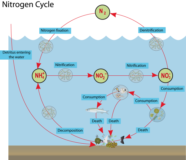
In both of these biogeochemistry labs, nitrogen isotopes (referred to as d15N, the ratio of the heavy 15N nuclide to the lighter 14N nuclide in a sample compared to that of a known standard) are used to track nitrogen cycling processes. The d15N of a water mass is a result of the relative proportions of different nitrogen cycling processes — nitrogen fixation, nitrogen assimilation, the rate of supply, the extent of nutrient utilization, etc. These can either be constrained directly via 15N tracer studies or can be inferred from “natural abundance” nitrogen isotopic composition, the latter of which will be used as a tool for this project.
On this cruise she has 3 sample types — phytoplankton, zooplankton, and seawater nitrate — and two overarching questions that these samples will address: How variable is “baseline d15N” along the entire eastern seaboard, and does this isotopic signal propagate to higher trophic levels? Each sample type gives us a different “timescale” of N cycling on the U.S. continental shelf. She will be filtering phytoplankton from various depths onto filters, she will be collecting seawater for subsequent analysis in the lab, and she will be collecting zooplankton samples — all of which will be analyzed for nitrogen isotopic composition (d15N).
Biogeochemistry background:
Biogeochemists look at everything on an integrated scale. We like to look at the box model, which looks at the surface ocean and the deep ocean and the things that exchange between the two.
The surface layer of the ocean: euphotic zone (approximately 0-150 m-but this range depends on depth and location and is essentially the sunlit layer); nutrients are scarce here.
When the top zone animals die they sink below the euphotic zone and into the aphotic zone (150 m-4000m), and the bacteria break down the organic matter into inorganic matter (nitrate (NO3), phosphate (PO4) and silicate (Si(OH)3.). In terms of climate, an important nutrient that gets cycled is carbon dioxide.We look at the nitrate, phosphate, and silicate as limiting factors for biological activity for carbon dioxide, we are essentially calculating these three nutrients to see how much carbon dioxide is being removed from the atmosphere and “pumped” into the deep sea. This is called the biological pump. Additionally, the particulate matter that falls to the deep sea is called Marine Snow, which is tiny organic matter from the euphotic zone that fuels the deep sea environments; it is orders of magnitude less at the bottom compared to the top.
Visual Representation of the aphotic and euphotic zones and the nutrients that cycle through them. Photo by: Patricia Sharpley
Did you know that the “Deep sea is really acidic, holds a lot of CO2 and is the biggest reservoir of C02 in the world?” – From Jessica Lueders- Demont, graduate student at Princeton.
One of the most important limiting factors for phytoplankton is nitrogen, which is not readily available in many parts of the global ocean. “A limiting nutrient is a chemical necessary for plant growth, but available in quantities smaller than needed for algae and other primary producers to increase their abundance. Organisms can grow and reproduce only when they have sufficient nutrients. For algae, the carbon source is CO2and this, at least in the surface water, has a constant value and is not limiting their growth. The limiting nutrients are minerals (such as Fe+2), nitrogen, and phosphorus compounds” (Patricia Sharpley 2010).
Conversely, phosphorus is the limiting factor on land. The most common nitrogen is molecular nitrogen or N2, which has a strong bond to break and biologically it is very expensive to fix from the atmosphere.
Biological, chemical, and physical oceanography all work together in this biogeochemistry world and are needed to have a productive ocean. For example, we need the physical oceanography to upwell them to the surface so that the life in the euphotic zone can use them.
Activities on the ship that I am assisting Jessica with:
Zooplankton collected using mini bongos with a 165 micron mesh and then further filtered at meshes: 1000, 500, and ends with 250 microns, this takes out all of the big plankton that she is not studying and leaves only her own in her size range which is 165-200 microns.
She is collecting zooplankton water samples because it puts the phytoplankton that she is focusing on into perspective.
The last of the mesh buckets that’s filtering for phytoplankton. Photo by: DJ Kast
Aspirator pump sucks out all of the water so that the zooplankton are left on a glass fiber filter (GFFs) on the filtration rack.
Aspirator pump that is on the side sucks out all of the air so that the plankton get stuck on the filters at the bottom of the cups seen here. Photo by: DJ Kast
Bottom of the cup after all the water has been sucked through. Photo by: DJ Kast
Jessica removing the filter with sterilized tweezers to place into a labeled petri dish. Photo by: DJ Kast
Labeled petri dish with GFF of phytoplankton on it. Photo by: DJ Kast
Video of this happening:
Phytoplankton filtering:
Jessica collecting her water sample from the Niskin bottle in the Rosette. Photo by DJ KastUp close shot of the spigot that releases water from Niskin bottle in the Rosette. Photo by DJ KastDJ Kast helping Jessica collect her 4 L of seawater from the Niskin bottle in the Rosette. Photo by Jerry P.DJ and Jessica collect her 4 L of seawater from the Niskin bottle in the Rosette. Photo by Jerry P.Chief Scientist Jerry Prezioso and Megan Switzer next to the CTD and Rosette Photo by: DJ Kast
May 21, 14:00 hours: Phytoplankton filtering with Jessica.
In addition to the small bottles Jessica needs, we filled 4 L bottles with water at the 6 different depths (100, 50, 30, 20, 10, 3 m) as well.
We then brought all the 4 L jugs into the chemistry lab to process them. The setup includes water draining through the tubing coming from the 4 L jugs into the filters with the GFFs in it. Each 4 L jug is filtered by 2 of these filter setups preferably at an equal rate. The deepest depth 100 m was finished the quickest because it had the least amount of phytoplankton that would block the GFF and then a second jug was collected to try and increase the concentration of phytoplankton on the GFF.
Phytoplankton filtration setup. Photo by DJ KastThe filter and pump setup up close. Photo by DJ KastUp close shot of the GFF within the filtration unit. Photo by DJ KastJessica keeping an eye on her filtration system to make sure nothing is leaking and that there are no air bubbles restricting water flow. Photo by DJ KastHere I am helping Jessica setup the filtration unit.Photo by Jessica Lueders- DumontThe GFF with the phytoplankton (green stuff) on it. Photo by: DJ Kast
There are 2 filters for each depth, and since she has 12 filtration bottles total, then she would be collecting data from 6 depths. She collects 2 filters so that she has replicates for each depth.
Here they are all laid out to show the differences in phytoplankton concentration.
The 6 depths worth of GFFs. See how the 30 m is the darkest. Thats evidence for the chlorophyll max. Photo by: DJ Kast
She will fold the GFF in half in aluminum foil and store it at -80C until back in the lab at Princeton. There, the GFF’s are combusted in an elemental analyzer and the resulting gases run through a mass spectrometer looking for concentrations of N2 and CO2. The 30 m GFF was the most concentrated and that was because of a chlorophyll maximum at this depth.
Chlorophyll maximum layers are common features of vertically stratified water columns. There is a subsurface maximum or layer of chlorophyll concentration. These are found throughout oceans, lakes, and estuaries around the world at varying depths, thicknesses, intensities, composition, and time of year.
NOAA Teacher at Sea Julia West Aboard NOAA ship Gordon Gunter March 17 – April 2, 2015
Mission: Winter Plankton Survey Geographic area of cruise: Gulf of Mexico Date: March 29, 2015
Weather Data from the Bridge
Time 1600; clouds 35%, cumulus; wind 170 (S), 18 knots; waves 5-6 ft; sea temp 24°C; air temp 23°C
Science and Technology Log
We have completed our stations in the western Gulf! Now we are steaming back to the east to pick up some stations they had to skip in the last leg of the research cruise, because of bad weather. It’s going to be a rough couple of days back, with a strong south wind, hence the odd course we’re taking (dotted line). Here’s the updated map:
Here’s where we are as of the afternoon of 3/29 (the end of the solid red line. We’ve connected all the dots!
I had a question come up: How many types of plankton are there? Well, that depends what you call a “type.” This brings up a discussion on taxonomy and Latin (scientific) names. The scientists on board, especially the invertebrate scientists, often don’t even know the common name for an organism. Scientific names are a common language used everywhere in the world. A brief look into taxonomic categories will help explain. When we are talking about numbers, are we talking the number of families? Genera? Species? Sometimes all that is of interest are the family names, and we don’t need to get more detailed for the purposes of this research. Sometimes specific species are of interest; this is true for fish and invertebrates (shrimp and crabs) that we eat. Suffice it to say, there are many, many types of plankton!
Another question asks what the plankton do at night, without sunlight. Phytoplankton (algae, diatoms, dinoflagellates – think of them like the plants of the sea) are the organisms that need sunlight to grow, and they don’t migrate much. The larval fish are visual feeders. In a previous post I explained that they haven’t developed their lateral line system yet, so they need to see to eat. They will stay where they can see their food. Many zooplankton migrate vertically to feed during the night when it is safer, to avoid predators. There are other reasons for vertical migration, such as metabolic reasons, potential UV light damage, etc.
Vertical migration plays a really important role in nutrient cycling. Zooplankton come up and eat large amounts of food at night, and return to the depths during the day, where they defecate “fecal pellets.” These fecal pellets wouldn’t get to the deep ocean nearly as fast if they weren’t transported by migrating zooplankton. Thus, migration is a very important process in the transport of nutrients to the deep ocean. In fact, one of the most voracious plankton feeders are salps, and we just happened to catch one! Salps will sink 800 meters after feeding at night!
Salp caught in the neuston sample. Salps are a colony of tunicates (invertebrate chordates for you biology students – more closely related to humans than shrimp are!)
Now it’s time to go back into the dry lab and talk about what happens in there. I’ll start with the chlorophyll analysis. In the last post I described fluorescence as being an indicator of chlorophyll content. What exactly isfluorescence? It is the absorption and subsequent emission of light (usually of a different wavelength) by living or nonliving things. You may have heard the term phosphorescence, or better yet, seen the waves light up with a beautiful mysterious light at night. Fluorescence and phosphorescence are similar, but fluorescence happens simultaneously with the light absorption. If it happens after there is no light input (like at night), it’s called phosphorescence.
An example of phosphorescence. We haven’t seen it yet, but I hope to! (From eco-adventureholidays.co.uk)
Well, it is not just phytoplankton that fluoresce – other things do also, so to get a more accurate assessment of the amount of phytoplankton, we measure the chlorophyll-a in our niskin bottle samples. Chlorophyll-a is the most abundant type of chlorophyll.
We put the samples in dark bottles. Light allows photosynthesis, and when phytoplankton (or plants) can photosynthesize, they can grow. We don’t want our samples to change after we collect them. For this same reason, we also process the samples in a dark room. I won’t be able to get pictures of the work in action, but here are some photos of where we do this.
This is the room where we do the chlorophyll readings.
We filter the chlorophyll out of the samples using this vacuum filter:
Each of these funnels filters the sea water through a very fine filter paper to capture the chlorophyll.
The filter papers are placed in test tubes with methanol, and refrigerated for 24 hours or so. Then the test tubes are put in a centrifuge to separate the chlorophyll from the filter paper.
Some of the test tubes for chlorophyll readings, and the filter paper. This box costs about $100!
The chlorophyll values are read in this fancy machine. Hopefully the values will be similar to those values obtained during the CTD scan. I’ll describe that next.
This fluorometer reads chlorophyll levels.
While the nets and CTD are being deployed and recovered, one person in the team is monitoring and controlling the whole event on the computer. I got to be this person a few times, and while you are learning, it is stressful! You don’t want to forget a step. Telling the winch operator to stop the bongos or CTD just above the bottom (and not hit bottom) is challenging, as is capturing the “chlorophyll max” by stopping the CTD at just the right place in the water column.
This is the graph that comes back from the SeaCAT on the bongo. We are interested in the green line, which shows depth as it goes down and comes back up.Here I am trying my hand at the computers. The monitor on the left is the live video of what is happening on deck (see the neuston net?). Photo by A.L. VanCampen
This is the CTD graph after it has been completed. The left (magenta) line is the chlorophyll, and the horizontal red lines are where we have fired a bottle and collected a sample. Notice the little spike partway down. That is the chlorophyll max, and we try to capture that when bringing it back up. The colored chart shows columns of continuous data coming in.
Here’s another micrograph of larval fish. Notice the tongue fish, the big one on the right. It is a flatfish, related to flounder. See the two eyes on one side of its head? Flatfish lie on the bottom, and have no need for an eye facing the bottom. When they are juveniles, they have an eye on each side, and one of the eyes migrates to the other side, so they have two eyes on one side! Be sure to take the challenge in the caption!
There is a cutlass fish just right of center. Can you find the other one? How about the lizard fish? Hint – look back at the picture in the last post. Photo credit Pamela Bond/NOAA
Personal Log
It’s time to introduce our intrepid leader, Commanding Officer Donn Pratt, known as CO around here. CO lives (when not aboard the Gunter) in Bellingham, WA. He got his start in boats as a kid, starting early working on crab boats. He spent 9 years with the US Coast Guard, where he had a variety of assignments. In 2001, CO transferred to NOAA, while simultaneously serving in the US Navy Reserve. CO is not a commissioned NOAA officer; he went about his training in a different way, and is one of two US Merchant Marine Officers in the NOAA fleet. He worked as XO for about seven years on various ships, and last year he became CO of the Gordon Gunter.
CO is well known on the Gunter for having strong opinions, especially about food and music. He loves being captain for fish research, but will not eat fish (nor sweet potatoes for that matter). A common theme of meal conversations is music; CO plays drums and guitar and is a self-described “music snob.” We have fun talking about various bands, new and old.
CO Don Pratt on the bridge.
One of the most experienced and highly respected of our crew is Jerome Taylor, our Chief Boatswain (pronounced “bosun”). Jerome is the leader of the deck crew. He keeps things running smoothly. As I watch Jerome walk around in his cheerful and hardworking manner, he is always looking, always checking every little thing. Each nut and bolt, each patch of rust that needs attention – Jerome doesn’t miss a thing. He knows this ship inside and out. He is a master of safety. As he teaches the newer guys how to run the winch, his mannerism is one of mutual respect, fun and serious at the same time.
Jerome has been with NOAA for 30 years now, and on the Gunter since NOAA acquired the ship in 1998. He lives right in Pascagoula, MS. I’ve only been here less than two weeks, but I can see what a great leader he is. When I grow up, I want to be like Jerome!
Chief Bosun Jerome Taylor, refusing to look at the camera. No, he’s not grilling steaks; he’s operating the winch!
Challenge Yourself!
OK, y’all (yes, I’m in the south), I have a math problem for you! Remember, in the post where I described the bongos, I showed the flowmeter, and described how the volume of water filtered can be calculated? Let’s practice. The volume of water filtered is the area of the opening x the “length” of the stream of water flowing through the bongo.
V = area x length.
Remember how to calculate the area of a circle? I’ll let you review that on your own. The diameter (not radius) of a bongo net is 60 cm. We need the area in square meters, not cm. Can you make the conversion? (Hint: convert the radius to meters before you calculate.)
Now, that flow meter is just a counter that ticks off numbers as it spins. In order to make that a usable number, we need to know how much distance each “click” is. So we have R, the rotor constant. It is .02687m.
R = .02687m
Here’s the formula:
Volume(m3) = Area(m2) x R(Fe – Fs) m
Fe = Ending flowmeter value; Fs = Starting flowmeter value
The right bongo net on one of the stations this morning had a starting flowmeter value of 031002. The ending flowmeter value was 068242.
You take it from here! What is the volume of water that went through the right bongo net this morning? If you get it right, I’ll buy you an ice cream cone next time I see you! 🙂
Sunset from the Gordon Gunter as we are heading east.
NOAA Teacher at Sea Julia West Aboard NOAA ship Gordon Gunter March 17 – April 2, 2015
Mission: Winter Plankton Survey Geographic area of cruise: Gulf of Mexico Date: March 27, 2015
Weather Data from the Bridge
Time 1300; clouds 10%, cirrus; wind 330° (NNW), 10 knots; air temp. 18°C; water temp. 22°C; wave height 1 ft.; swell height 2-3 ft.
Science and Technology Log
We had some high winds (25 knots) these past couple of days, and the seas got too rough to work. Last night we headed closer to shore to find calmer water, and all ops were called off. Today we are back on (a new) course! Here’s the map with our rerouted course on it:
Plankton sampling stations covered through 3/27/15
I want to start off this post answering two really good questions that have come up. Why do we send the samples all the way to Poland, only to have the data and some specimens come right back here? Is that typical U.S. outsourcing? Well, I had heard a rumor, and now I have a definitive answer about that, and it’s rather interesting! I had no idea I’d be learning history lessons on this journey, but this post has two important events in history.
If you have studied World War II, you may have heard of the Marshall Plan, otherwise known as the European Recovery Program, where the U.S. provided grants and loans for the rebuilding of war-ravaged European countries. Poland needed to pay off their war debt to the U.S., and the U.S. had a need. Here’s what I learned:
“The ‘father of the Polish Sorting Center’, Ken Sherman, visited a number European counties participating in the Marshall Plan looking for one that would be interested in setting up a Plankton Sorting and Identification Center. Poland was the one that took him up on the offer. Actually the leader of the Province of Pomerania in western Poland saw the economic possibilities for his state and thus was born the U.S.-Poland Agreement. By the way, the agreement lasted the entire time Poland was an eastern block country under the domination of the old Soviet Union. That in itself is a remarkable tale!” Information courtesy of Joanne Lyczkowski-Shultz, renowned Plankton scientist.
There you have it. Who knew? I think debt is paid off, but we have a great working relationship with the Polish Sorting Center, and they are good at what they do, so we continue.
Another good question was, why do we sample every year? Do the samples change? The reason is because just like for so many things (think of climate change as an example), it is by monitoring long term that we get the big picture and see change, if it is occurring. I asked if the samples change over time, but the answer isn’t known among the scientists on this ship. There are other departments that analyze the data; these scientists specialize in collecting it.
Today I want to introduce the CTD (Conductivity, Temperature, and Depth) unit. This expensive (think $20,000 and up) piece of equipment provides a hefty amount of data about the water column in our 200 meter sampling range. This is the last unit we deploy when we get to a station, after the neuston net comes back on board. Here’s what it looks like (the actual CTD part is on the bottom):
The CTD unit being lowered into the water.
Here we are bringing the CTD back on board
Here are some close-up pictures:
There are 3 niskin bottles on the unit now (one not visible). It can hold 12.
The niskin bottles collect samples of water at whatever depth we determine. They are lowered into the water with both ends open (see the top and bottom lids are cocked open), so water flows through them. When they get to a certain depth, we can “fire” a bottle, and an electric signal trips a little lever at the top, and the top and bottom lids spring shut. We collect samples at the surface, at the bottom of the photic zone (200 meters or the ocean floor if we can’t go that deep), and at whatever place in the water column there is the maximum amount of chlorophyll. How do we know that, you should be wondering? Well, that’s where this unit comes in. This is officially the CTD – the expensive part:
The CTD is the “brains;” it does all the technical work.
It’s hard to see because it is on a black mat. The CTD sends constant information back to our computers. Water is pumped through the unit (see the tubing?) It is recording temperature, depth (by water pressure), oxygen level, salinity, turbidity (water clarity) and fluorescence. The conductivity, or the ability to pass an electric current, gives a measure of the dissolved salts in the water, or salinity (there’s chemistry and physics for you!) Fluorescence is one indicator of chlorophyll content. If you have learned about photosynthesis, it is chlorophyll in plant leaves that absorbs the sunlight and makes a plant green. The chlorophyll, therefore, is an indicator of the phytoplankton, such as single-celled algae, that are in the water. Remember, some zooplankton (mostly the invertebrates) eat phytoplankton, and most of our baby fish eat the zooplankton, so it’s good to know what is going on at the base of the food chain.
All of these things create cool little lines on a graph as the CTD is lowered. After capturing water at the bottom, we bring it up to approximately what the chlorophyll maximum was on the way down, by watching the data feed as it comes in, and fire another bottle to grab a sample of that water. Then we do it again at the surface.
So far I’ve shared what we do on the deck – how we collect the samples. In another post I will share with you what all this stuff looks like in the lab on the computer screen. Remember I said there is constant communication between the lab, the bridge, and the deck? Well, in the lab (but not the deck) we know exactly where the bottom is, and we have to give the order to stop the descent of the CTD (or bongos). “All stop!” is the command on the radio. “All stop,” the winch operator repeats as he stops the winch. If conditions are not right, the bridge or the scientists can put off or call off a deployment. We had some strong winds and high seas these past couple of days, so working with flying nets can get dangerous. The neuston is the first to get cancelled – that’s a big net!
In the next few blog posts I’m going to share with you some micrographs (pictures taken through a microscope) of what we’ve been catching. It is awe-inspiring to see all these little specks that fill our sieves close up!
Again, here’s what they look like in a jar:
This is a nice sample from one of the bongo nets. Lots of little guys in there!
And here’s what happens when they are sorted under a microscope:
These are all larval fish. Top left: lizard fish. The bigger one in center is cutlass fish. These are both 8-9mm long. Photo courtesy of Pamela Bond, NOAA.
Personal Log
The other day we saw pilot whales from the bridge. It was pretty cool – they were right in front of the ship. If it was a kind of slow moving whale, we would have slowed down to avoid hitting them, but pilot whales move fast, and got out of our way easily. I didn’t get pictures – sorry! But here is somebody who was taking refuge on the deck:
Yellow-crowned night heron taking a rest.
Sometimes birds get blown off course, or get tired while crossing a big expanse of water. We had two big cattle egrets sitting up high on the deck a few days ago. And often songbirds land on deck, completely exhausted.
We had another fire drill and abandon ship drill; these happen once a week. This time we practiced crawling (because smoke rises) to the nearest exit with our eyes shut.
Here I am feeling my way to the exit. Photo credit: A.L. VanCampenEveryone gathers on deck with their survival suits (and hats required) in the abandon ship drill
Here’s a random picture that I took. Occasionally we get plastic in our nets, and all this is recorded, of course. But if a man o’war is plankton, and this mylar balloon acts like plankton, is it plankton?
No, it’s pollution!
I’d like to introduce Tony VanCampen, our Electronics Technician (ET). Without him, operations would come to a stop around here. Tony is in charge of all the electronics on the ship. That includes things like the SeaCAT, the CTD, the computers, the radar, radios, GPS, meteorology gear, the internet connection….to name a few. Tony says “ET” stands for “Everything Tech.”
Our internet! VSAT (Very Small Aperture Terminal) – this is how I am posting to this blog.
Tony spent 20 years in the US Navy before joining NOAA. He spent 6 years on the USS Berkeley in the Pacific, followed by a couple of years of shore duty, during which time he went back to school to learn all the new equipment that was being used on the new ships. In 1994, Tony started a new tour on the brand new Navy ship USS Cole. He was on two deployments of the USS Cole. Where were you on October 12, 2000 – were you even born yet? Tony was on the Cole, in Yemen, when two men in a normal looking small boat came up to the ship, waved, and then blew themselves up, destroying a section of the Cole and killing 17 sailors and injuring another 40+. Tony was not visibly injured, but we now know that PTSD (Post Traumatic Stress Disorder) is a very real and serious affliction. Tony thought he was doing well until Sept. 11, 2001, when he and his wife realized he was not well at all. He credits his family and friends for seeking help and saving his life.
Why do I mention this? Because you never know, when you go to a new place, what the people you meet have been through. How important it is to remain sensitive and raise awareness of PTSD! Thanks to Tony for his willingness to share his story and thanks to those men and women who serve our country.
Tony VanCampen, ET
Tony, in the mood to dress like a minion.
Lastly, here are a few pictures from our day with 5-7 foot seas. I have not been seasick – yay!
Big waves from the lower deck as we were trying to sample.Gorgeous!The day ends.
NOAA Teacher at Sea Lauren Wilmoth Aboard NOAA Ship Rainier October 4 – 17, 2014
Mission: Hydrographic Survey Geographical area of cruise: Kodiak Island, Alaska Date: Sunday, October 12, 2014
Weather Data from the Bridge Air Temperature: 1.92 °C
Wind Speed: 13 knots
Latitude: 58°00.411′ N
Longitude: 153°10.035′ W
Science and Technology Log
The top part of a tidal station. In the plastic box is a computer and the pressure gauge.
In a previous post, I discussed how the multibeam sonar data has to be corrected for tides, but where does the tide data come from? Yesterday, I learned first hand where this data comes from. Rainier‘s crew sets up temporary tidal stations that monitor the tides continuously for at least 30 days. If we were working somewhere where there were permanent tidal station, we could just use the data from the permanent stations. For example, the Atlantic coast has many more permanent tidal stations than the places in Alaska where Rainier works. Since we are in a more remote area, these gauges must be installed before sonar data is collected in an area.
We are returning to an area where the majority of the hydrographic data was collected several weeks ago, so I didn’t get to see a full tidal station install, but I did go with the shore party to determine whether or not the tidal station was still in working condition.
A tidal station consists of several parts: 1) an underwater orifice 2) tube running nitrogen gas to the orifice 3) a nitrogen tank 4) a tidal gauge (pressure sensor and computer to record data) 5) solar panel 6) a satellite antennae.
Let me explain how these things work. Nitrogen is bubbled into the orifice through the tubing. The pressure gauge that is located on land in a weatherproof box with a laptop computer is recording how much pressure is required to push those bubbles out of the orifice. Basically, if the water is deep (high tide) there will be greater water pressure, so it will require more pressure to push bubbles out of the orifice. Using this pressure measurement, we can determine the level of the tide. Additionally, the solar panel powers the whole setup, and the satellite antennae transmits the data to the ship. For more information on the particulars of tidal stations click here
Tidal station set-up. Drawing courtesy of Katrina Poremba.Rainier is in good hands.
The tidal station in Terror Bay did need some repairs. The orifice was still in place which is very good news, because reinstalling the orifice would have required divers. However, the tidal gauge needed to be replaced. Some of the equipment was submerged at one point and a bear pooped on the solar panel. No joke!
After the tidal gauge was installed, we had to confirm that the orifice hadn’t shifted. To do this, we take manual readings of the tide using a staff that the crew set-up during installation of the tidal station. To take manual (staff) observations, you just measure and record the water level every 6 minutes. If the manual (staff) observations match the readings we are getting from the tidal gauge, then the orifice is likely in the correct spot.
Just to be sure that the staff didn’t shift, we also use a level to compare the location of the staff to the location of 5 known tidal benchmarks that were set when the station was being set up as well. As you can see, accounting for the tides is a complex process with multiple checks and double checks in place. These checks may seem a bit much, but a lot of shifting and movement can occur in these areas. Plus, these checks are the best way to ensure our data is accurate.
ENS Micki and LTJG Adam setting up the staff, so the surveyor can make sure it hasn’t moved.Mussels and barnacles on a rock in Terror Bay.Leveling to ensure staff and tidal benchmarks haven’t moved.
Today, I went to shore again to a different area called Driver Bay. This time we were taking down the equipment from a tidal gauge, because Rainier is quickly approaching the end of her 2014 season. Driver Bay is a beautiful location, but the weather wasn’t quite as pretty as the location. It snowed on our way in! Junior Officer Micki Ream who has been doing this for a few years said this was the first time she’d experienced snow while going on a tidal launch. Because of the wave action, this is a very dynamic area which means it changes a lot.
In fact, the staff that had been originally used to manually measure tides was completely gone, so we just needed to take down the tidal gauges, satellite antenna, solar panels, and orifice tubing. The orifice itself was to be removed later by a dive team, because it is under water. After completing the tidal gauge breakdown, we hopped back on the boat for a very bumpy ride back to Rainier. I got a little water in my boots when I was hopping back aboard the smaller boat, but it wasn’t as cold as I had expected. Fortunately, the boat has washers and driers. It looks like tonight will be laundry night.
Driver Bay
Personal Log
The food here is great! Last night we had spaghetti and meatballs, and they were phenomenal. Every morning I get eggs cooked to order. On top of that, there is dessert for every lunch and dinner! Don’t judge me if I come back 10 lbs. heavier. Another cool perk is that we get to see movies that are still in the theaters! They order two movies a night that we can choose from. Lastly, I haven’t gotten seasick. Our transit from Seward to Kodiak was wavy, but I don’t think it was as bad as we were expecting. The motion sickness medicines did the trick, because I didn’t feel sick at all.
Did You Know?
NOAA (National Oceanic and Atmospheric Administration) contains several different branches including the National Weather Service which is responsible for forecasting weather and issuing weather alerts.


