So, we’ve taken a chilly dive into the why behind the focus on the pollock. Today, I will take you into “The Cave,” where we can learn how scientists use sound to locate and count pollock. On the port side of the main deck sits a dark, windowless room lit only by the dozen or so monitors adorning its aft wall. A gentle, constant humming fills the room from racks and racks of electronics, servers, and support equipment that dominate the center of this space. While the OOD on the bridge steers this vessel, “The Cave” calls the scientific shots by determining the ship’s course as well as the timing and location of all science operations.
Abigail McCarthy and Mike Levine discuss plans for the day shift. Time at sea is precious; this vessel operates 24/7 in all conditions. For the past two days, a very quiet, fishless northern extension has limited opportunities. But remember, even a null result is a result!
Acoustics 101
Since the early 20th century, scientists have used the unique ability of sound waves to transmit very efficiently through water for remote sensing. “Pings” of acoustic energy are generated by a transmitter, and then the backscatter (or reflected sound) is detected by a receiver. Early pioneers used sonar to better understand the physical geography of ocean basins in a process called bathymetry.
USS Stewart first tested an early form of echosounder in 1922 as part of preparations for the installation of the Transatlantic cable.
Not long after the first echosounders made their way aboard ships, scientists realized that as the quality of the instrument increased, they could measure the backscatter (or reflected sound) off of other objects besides the seafloor. Large backscattering layers far above the seafloor were targeted by fishing vessels using the new technology, demonstrating the effectiveness of echosounders at locating marine organisms throughout the water column.
Early innovators in Norway and England reported success in using echosounders to detect large schools of fish and began actively monitoring their behavior (Balls, 1948).
The following decades of acoustic research relied on analog, single-beam systems, which were often towed behind or below a vessel and recorded a narrow swath directly below the ship onto a paper echogram.
A 3d porcelain rendering of this now-famous echogram (the recorded chart of an echosounder) from the Shelikof Straight adorns the entry to the NOAA Alaska Fisheries Science Center in Seattle. The strong red and yellow reflections that sweep gently across the bottom represent the strong backscatter from the seafloor, and the large red cloud represents a large school of pollock.
The 1990’s welcomed a new era in echosounder technology with the release of the SIMRAD EK-500. This landmark digital echosounder combined multi-frequency operation with improved data processing and integration tools, enabling much better estimates of fish population density and biomass.
Larger acoustic targets, such as the swim bladder of a large fish, produce strong backscatter at relatively low frequencies, whereas smaller organisms, such as krill and copepods, reflect sound only at much higher frequencies. Multi-frequency echo sounder measurements allow scientists to discriminate between acoustic targets of different sizes and target strengths and more accurately estimate the biomass of individual organisms as they scroll across the screen.
Next time, we will look at the echograms produced aboard Oscar Dyson and receive a crash course in interpretation from the Cave!
Personal Log
Work hard, play hard is an unofficial motto aboard Oscar Dyson. The officers, crew, and science team are keeping a fierce eye on the World Cup when off duty (Colombia’s goal call-back was a travesty!!).
The “Inaugural Collin McMillan Memorial Biannual Oscar Dyson Amateur Cribbage Tournament” is underway; stay tuned for updates and potential video coverage of the championship match!The future gyotaku model, Northern rock sole (Lepidopsetta polyxystra), posing for a picture before her big debut.Gyotaku is the traditional Japanese art of collecting fish prints. Engineer Victoria Southwick, ENS Josh Bennett, and Lt. Jesse Pierce captured the print of a Northern rock sole (Lepidopsetta polyxystra) brought up on haul 71, 06/28/26.
Wildlife sightings
A Short-tailed albatross (Phoebastria albatrus) follows us during trawling operations, hoping for a fishy treat. This threatened marine bird is a tale of cautious conservation success. Their population in the 1950s dwindled to as low as 25 individuals. Today, roughly 4,200 individuals are known to exist.
Fun Fact
In the Cave, it is not uncommon for the shallow layer to be filled with a mix of non-fish backscatter. Everyone has their pet theories as to what may be the source of these shallow acoustic targets (we know they aren’t fish), but they have all agreed to call it by one name… munge. Below is my artist’s interpretation of Munge as a heavy metal album.
MUNGE album cover
Sources
Balls, R. 1948. Herring fishing with the echometer. Journal du Conseil International pour l’Exploration de la Mer, 15: 193–206.
Korneliussen, R. J. (2018). Acoustic target classification.
Benoit-Bird, K. J., & Lawson, G. L. (2016). Ecological insights from pelagic habitats acquired using active acoustic techniques. Annual review of marine science, 8, 463-490.
Mordy, C. W., Bond, N. A., Cokelet, E. D., Deary, A., Lemagie, E., Proctor, P., … & Wisegarver, E. (2023). Progress of fisheries-oceanography coordinated investigations in the Gulf of Alaska and Aleutian Passes. Oceanography, 36(2/3), 94-100.
De Robertis, A., McKelvey, D. R., & Ressler, P. H. (2010). Development and application of an empirical multifrequency method for backscatter classification. Canadian Journal of Fisheries and Aquatic Sciences, 67(9), 1459-1474.
Simmonds, J., & MacLennan, D. N. (2008). Fisheries acoustics: theory and practice. John Wiley & Sons.
Holliday, D. V., & Pieper, R. E. (1995). Bioacoustical oceanography at high frequencies. ICES Journal of marine Science, 52(3-4), 279-296.
Mission: Acoustic Trawl Survey (Leg 3 of 3) Geographic Area of Cruise: Pacific Ocean/ Gulf of Alaska Date: Sunday, August 13, 2023
Weather Data Lat 59.12 N, Lon 150.11 W Sky condition: Partly Cloudy Wind Speed: 13 knots Wind Direction: 330° Air Temp: 14 °C
Science and Technology blog
The ocean is a really big place. We have really only mapped about 5% of the ocean bottom. How do we manage fisheries if we have to count fish in an area that is overwhelmingly large? This is where the genius of acoustics and trawl sampling complement each other. The scientists aboardNOAA Ship Oscar Dyson use the echo sounders to find fish or other animals lurking in the ocean and then they can extrapolate and upscale that data to a much larger area which is covered by their transects.
Wait! That is a lot of information using language that folks don’t really use at the dinner table. Could you please explain this in more basic terms? You bet, as a matter of fact in the last couple of days I have been swimming in a sea of new vocabulary, talking to really smart people and trying to keep up with the conversation that it almost makes my head explode. Don’t worry, I am safe. But it’s really impressive how scientists have developed ways to accurately know fish and marine organism populations in the ocean with out having to sample all of it.
Acoustics
Acoustics uses the echo-sounders a lot like a fish finder, but the ones on NOAA Ship Oscar Dyson are much more capable than the type you would find on your boat. The echo-sounders are attached to the bottom of a lowered centerboard—essentially a large keel—in the center of the boat, and they measure five different frequencies with different wavelengths.
View of the 5 different frequencies measured by the echosounders, one in each frame. The darker marks on the screen could be fish, jellyfish, krill or other marine organisms, this is referred to as “backscatter.” The red circles show the different frequencies used to measure the backscatter.
So, if we can see the fish using acoustics, why do scientists need to sample using a trawl net? As you can see above, the marks in the backscatter can show the depth and the approximate shape of objects, but there is not enough detail to tell exactly what kind of organism is present. Most of the scientists on board have a pretty good idea what kind of fish or organisms are present, but the most definitive way to know is to take a trawl sample.
Trawl Sampling
The trawl net as seen in the picture below is being set off the aft deck.
The part that is in the air is called the codend. That is the section of the net where the specimens are ultimately collected.
The trawl is a about 172 meters long and it stored on these rollers on the back deck.
When the trawl is deployed to the depth that the scientists want to sample, the net will funnel fish and other organisms into it. This is called flying the net.
The screen above diagrams three different views of the net as it is pulled through the water. You can see that the trawl net was not directly behind the boat and went to a depth of 21.5 m.
In this image you can see the net and how far back it trails behind the Oscar Dyson.
I just have to include one more view of the trawl net from the bridge as it is pulled behind the boat.
This image was taken when the crew was bringing the net back into the boat, so the depth is shallower.
The next image shows the path that the net was pulled through the water.
The acoustics show the backscatter which the scientists make the trawl target. The next step is to process what is captured in the codend of the trawl and see exactly what is present.
Because the trawl is dragged through the water, it catches different organisms at different times. The scientists want to know when the different organisms were caught so they have cleverly attached a camera to the side of the net. Through the camera they can see which type of fish came into the trawl. Ultimately, this links the kind of acoustic backscatter viewed in the echograms recorded during the trawl to exactly the type of organism caught by the trawl.
The camtrawl: a camera that records the type of fish entering the net and when they enter.
Below is a picture of some fish as they enter the trawl net and move towards the codend.
The camera is looking across the net as the fish move past. The fish in the picture are pollock, the type of fish we are looking for on this leg of the cruise.
Transect Lines
So how do scientists take this information and extrapolate the data to a broader area? While the Oscar Dyson is out at sea they run transect lines while recording acoustic data. Transect lines are specific paths in the ocean. The picture below shows the transect lines that we plan to do and have done on this leg of the cruise.
The red lines are the transects we have done and the blue lines are the transects scientists plan to do in the remainder of this leg of the cruise. If you look closely there are pictures of fish symbols on the transect lines where the ship has made trawl samples.
Using the acoustic data that the echo-sounders provide and verifying the types of fish and other marine organisms through the trawl sampling allows the scientists to predict, with a high level of certainty, the amount and types of marine organisms that are present along the transect lines that were not trawl-sampled. Thus saving the taxpayers money, and allowing fisheries managers to use good data, keeping the fishery viable, and allowing commercial fishing boats to have reasonable catch limits.
Scientist in the Spotlight
Honestly it takes a team to make all of this happen. But, half of our team is sleeping at the moment, I have the night shift from 4pm to 4am, so I am going to introduce one fabulous expert in acoustics and fisheries:
Abigail McCarthy in the Acoustics Lab
Abigail McCarthy has been working for MACE: Midwater Assessment and Conservation Engineering Program since 2007. She received her undergraduate degree in Biology from Wellesley College and then obtained a Masters in Fisheries from Oregon State University.
For fun, she surfs and enjoys long-distance prone paddle board races. She has recently found a new love with fly fishing.
Aboard the Ship Oscar Dyson, she is working as a specialist helping to run the acoustics lab.
I asked Abigail what she thought of about her educational experience? She immediately said, “I love learning! High school and college were both a lot of fun.”
What would be a good suggestion for a young aspiring high school student pursuing a degree related to ocean studies or science in general?
Her response was great: “Being curious and working hard is more important than being brilliant. Persistence and determination will get you where you want to be in the future.” Finally, “Learn to code! Become familiar with programing languages like Python and R.”
Hopefully, I answered your burning questions about the use of acoustic trawl sampling, and surveys. Yet, there is so much more to learn. Why not take a trip yourself? Check NOAA’s website out and just apply.
Mission: 2023 Summer Acoustic-Trawl Survey of Walleye Pollock in the Gulf of Alaska
Geographic Area of Cruise: Islands of Four Mountains area, to Shumagin Islands area Location (2PM (Alaska Time), June 18): 55o 15.3391′ N, 160o 17.8682′ W
Data from 2PM (Alaska Time), June 18, 2023 Air Temperature: 8.9 oC Water Temperature (mid-hull): 7.7oC Wind Speed: 4 knots Wind Direction: 182 degrees Course Over Ground (COG): 356 degrees Speed Over Ground (SOG): 12 knots
Date: June 19, 2023
Acoustic fisheries surveys seek to estimate the abundance and distribution of fish in a particular area of the ocean. In my case, this Summer Survey is looking at walleye pollock in the Gulf of Alaska. How is this accomplished? Well, it’s not through this method:
The Alaska walleye pollock is widely distributed in the North Pacific Ocean with the largest concentrations in the eastern Bering Sea. For this expedition, Oscar Dyson is traveling to specific regions in the Gulf of Alaska and running transects perpendicular to the bathymetry/contours (which are not always perpendicular to the shore) to take measurements using acoustics and targeted trawling to determine the abundance and distribution of walleye pollock which informs stock assessment and management models. For this blog post, let’s focus on how and why we can use acoustics to locate fish.
Walleye pollock (Gadus chalcogrammus) are distributed broadly in the North Pacific Ocean and eastern and western Bering Sea. In the Gulf of Alaska, pollock are considered as a single stock separate from those in the Bering Sea and Aleutian Islands. Image from Alaska Department of Fish and Game.An snapshot of a nautical chart with transects plotted. The first transect was run during Leg 1 on June 14 at the furthest location to the west, then the ship worked its way back east with approximately 40 nautical miles between transects. Once Oscar Dyson reached the Shumagin Islands, survey work shifted into this area..
Our story starts with the fish itself. Alaska walleye pollock have a swim bladder. The swim bladder is an internal organ filled with gas that allows a fish to maintain its buoyancy and stability at depth.
One interesting effect of the swim bladder is that it also functions as a resonating chamber that can produce and receive sound through sonar technology. This connection was first discovered in the 1970s, when low-frequency sound waves in the ocean come in contact with swim bladders and they resonated much like a tuning fork and return a strong echo (see WHOI’s Listening for Telltale Echoes from Fish).
Internal anatomy of a boney fish. From Wikipedia (CC BY-SA 3.0).
The sound pulses travel down into the water column, illustrated by the white cones here, and bounce back when encountering resistance.(from NOAA Fisheries)
NOAA Fisheries uses echo sounding, which works by emitting vertical pulses of sound (often referred to as pings), and measuring the return strength and recording the time for the signal to leave and then return. Anything having a different density from the surrounding water (in our case – fish, plankton, air bubbles, the seafloor) can return a signal, or “echo”.
The strength or loudness of the echo is affected by how strongly different ocean elements reflect sound and how far away the source of the element is. The seafloor usually makes the strongest echo because it is composed of rock which has a density different than the density of water. In fish, the swim bladder provides a contrast from the water. In addition, each fish species has a unique target strength or amount of sound reflected to the receiver. The size and shape of the swim bladder influence the target strength. There is a different target strength to length relationship for each species of fish – the larger the fish, the greater the strength of the returning echo.
It’s important to note that echo sounders cannot identify fish species, directly or indirectly. The only way we know which fish species is causing a signal is based on trawl catch composition. There is nothing within the acoustic data that lets us identify fish species, even with the catch data. This is a subtle, but important, distinction. Acoustic data, particularly calibrated acoustic data, in tandem with the information from the trawl, definitely allows us to count fish.
Where is the echo sounder on Oscar Dyson? Look at the figure in the next section of this post – it’s a sketch of NOAA Ship Rainier, but the placement of the echo sounder is the same for Dyson. You can see a rectangular “board” that is extended down from the center of the ship. This is called – what else – the center board! Attached to the bottom of the center board are the echo sounders. When lowered, the echo sounders sit at 9 meters below the level of the sea (~4 meters below the bottom hull of the ship).
Did you know… Southern Resident killer whales use their own echolocation clicks to recognize the size and orientation of a Chinook’s swim bladder? Researchers report that the echo structure of the swim bladders from similar length but different species of salmon were different and probably recognizable by foraging killer whales. (reported in Au et al., 2010)
It starts with a calibration
Typical setup of the standard target and weight beneath the echo sounder.(from NOAA Fisheries)
Before we can begin collecting data, we need to calibrate the echo sounder. The calibration involves a standard target (a tungsten carbide sphere) with a known target strength. The calibration needs to be completed in waters that are calm and without significant marine life for the best results.
The sphere is suspended below the ship’s hull using monofilament lines fed through downriggers attached to ship railings. One downrigger is in line with the echo sounder on the starboard side, and the other two on the port side. This creates a triangle that suspends the sphere in the center of the echo sounder’s sound beam. By tightening and loosening the lines, the sphere can be positioned under the center of the sound beam and can also be moved throughout the beam. By doing an equipment calibration at the beginning and end of a survey, we can ensure the accuracy of our data.
One of the port side downriggers
A weight that goes at the bottom of the filament to ensure the calibration sphere remains below the echo sounder
The tungsten carbide sphere attached to the line, being lowered over the side
Latitude & Longitude: 43◦ 53.055’ N 124◦ 47.003’W Windspeed: 13 knots Geographic Area: @10-15 miles off of the Oregon/California coast Cruise Speed: 12 knots Sea Temperature 20◦Celsius Air Temperature 68◦Fahrenheit
Is this you?
Navigation is how Fairweather knows its position and how the crew plans and follows a safe route. (Remember navigation from the last post?) But what “drives” where the ship goes is Hydrographic survey mission. There is a stunning amount of sea floor that remains unmapped, as well as seafloor that has not been mapped following a major geological event like an earthquake of underwater volcano.
Why is Hydrography important? As we talked about in the previous post, the data is used for nautical safety, creating detailed maps of the ocean floor, setting aside areas are likely abundant undersea wildlife as conservation areas, looking at the sea floor to determine if areas are good for wind turbine placement, and most importantly to the residents off the Pacific coast, locating fault lines — especially subduction zones which can generate the largest earthquakes and cause dangerous tsunamis.
In addition to
generating the data needed to update nautical charts, hydrographic surveys
support a variety of activities such as port and harbor maintenance (dredging),
coastal engineering (beach erosion and replenishment studies), coastal zone
management, and offshore resource development. Detailed depth information and
seafloor characterization is also useful in determining fisheries habitat and
understanding marine geologic processes.
The history of hydrographic surveys dates back to the days
of Thomas Jefferson, who ordered a
survey of our young nation’s coast. This began the practice and accompanying sciences
of the coastal surveys. The practice of
surveys birthed the science of Hydrography (which we are actively conducting
now) and the accompanying science of Bathymetry (which we will go into on the
next post.) This practice continues of
providing nautical charts to the maritime community to ensure safe passage into
American ports and safe marine travels along the 95,000 miles of U.S. Coastline.
Want to learn more about Hydrographic Survey history? Click on THIS LINK for the full history by the NOAA.
Scientists have tools or equipment that they use to successfully carry out their research. Let’s take a look at a few of the tools hydrographic survey techs use:
Want to learn more about the science of SONAR? Watch the video below.
ps://www.youtube.com/watch?v=8ijaPa-9MDs
On board Fairweather (actually underneath it) is the survey tool call a TRANSDUCER which sends out the sonar pulses.
Multibeam sonar illustration
The transducer on Fairweather is an EM 710- multibeam echo sounder which you can learn more about HERE.
The Transducer is located on the bottom of the ship and sends out 256 sonar beams at a time to the bottom of the ocean. The frequency of the 256 beams is determined by the depth from roughly 50 pings per second to 1 ping every 10 seconds. The active elements of the EM 710 transducers are based upon composite ceramics, a design which has several advantages, which include increased bandwidth and more precise measurements. The transducers are fully watertight units which should give many years of trouble-free operation. This comes in handy since the device in on the bottom of Fairweather’s hull!
Here is the transducer on one of the launches:
View of transducer on a survey launch
The 256 sonar beams are sent out by the transducer simultaneously to the ocean floor, and the rate of return is how the depth of the ocean floor is determined. The rate of pulses and width of the “swath” or sonar beam array is affected by the depth of the water. The deeper the water, the larger the “swath” or array of sonar beams because they travel a greater distance. The shallower the water, the “swath” or array of sonar beams becomes narrower due to lesser distance traveled by the sonar beams.
The minimum depth that this transducer can map the sea floor is less than 3 meters and the maximum depth is approximately 2000 meters (which is somewhat dependent upon array size). Across track coverage (swath width) is up to 5.5 times water depth, to a maximum of more than 2000 meters. This echo sounder is capable of reaching deeper depths because of the lower frequency array of beams.
The transmission beams from the EM 710 multibeam echo sonar are electronically stabilized for roll, pitch and yaw, while they receive beams are stabilized for movements. (The movement of the ship) What is roll, pitch, and yaw? See below – these are ways the Fairweather is constantly moving!
Roll, Pitch, and Yaw
Since the sonar is sent through water, the variable of the water
that the sonar beams are sent through must be taken into account in the
data.
Some of the variables of salt water include: conductivity
(or salinity) temperature, depth, and density.
Hydrographic scientists must use tools to measure these factors in sea water, other tools are built into the hydrographic survey computer programs.
One of the tools used by the hydrographic techs is the XBT or Expendable Bathy Thermograph that takes a measurement of temperature and depth. The salinity of the area being tested is retrieved from the World Ocean Atlas which is data base of world oceanographic data. All of this data is transmitted back to a laptop for the hydrographers. The XBT is an external device that is launched off of the ship to take immediate readings of the water.
Launching the XBT: There is a launcher which has electrodes on it, then you plug the XBT probe to the launcher and then XBT is launched into the ocean off of the back of the ship. The electrodes transmit data through the probe via the 750-meter copper wire. The information then passes through the copper wire, through the electrodes, along the black wire, straight to the computer where the data is collected. This data is then loaded onto a USB then taken and loaded into the Hydrographic data processing software. Then the data collected by the XBT is used to generate the sound speed profile, which is sent to the sonar to correct for the sound speed changes through the water column that the sonar pulses are sent through. The water column is all of the water between the surface and seafloor. Hydrographers must understand how the sound moves through the water columns which may have different densities that will bend the sound waves. By taking the casts, you are getting a cross section “view” of the water column on how sound waves will behave at different densities, the REFRACTION (or bending of the sound waves) effects the data.
See how the XBT is launched and data is collected below!
Hydrotech Bekah Gossett preparing to cast
The XBT probe
The XBT launcher
I got to do a cast- thanks Bekah!
Instant readings from the XBT
Bekah downloading data from the XBT
Videos coming soon!
The other tool is the MVP or moving vessel profiler which takes measurements of conductivity, temperature, and depth. These are all calculated to determine the density of the water. This is a constant fixture on the aft deck (the back of the ship) and is towed behind the Fairweather and constantly transmits data to determine the speed of sound through water. (Since sonar waves are sound waves.)
MVP (left) and the launching wench (right)
The sonar software uses this data to adjust the calculation of the depth, correcting for the speed of sound through water due to the changes in the density of the ocean. The final product? A detailed 3d model of the seafloor!
Our current survey area! (Thanks Charles for the image!)
All of this data is run through the survey software. See screen shots below of all the screens the hydrographers utilize in the course of their work with explanations. (Thanks Sam!) It’s a lot of information to take in, but hydrographic survey techs get it done 24 hours a day while we are at sea. Amazing! See below:
Hydrographic Survey “Mission Control”
HYPACK Acquisition Software
Real time coverage map
Did You Know? An interesting fact about sonar: When the depth is deeper, a lower frequency of sonar is utilized. In shallower depths, a higher sonar frequency. (Up to 900 meters, then this rule changes.)
Question of the Day: Interested
in becoming a hydrographic survey tech?
See the job description HERE.
Challenge yourself — see if you can learn and apply the new terms and phrases below and add new terms from this blog or from your research to the list!
Geographic Area of Cruise: Northwest Pacific Ocean, off of the coast of Oregon
Date: July 31, 2017
Weather Data from the Bridge
Latitude: 44 49.160 N
Longitude 124 26.512
Temperature: 59oF
Sunny
No precipitation
Winds at 25.45 knots
Waves at 4-5ft
Science and Technology Log
Inside the acoustics lab
The scientists on the Hake survey project are constantly trying to find new methods to collect data on the fish. One method used is acoustics. Scientists Larry Hufnagle and Dezhang Chu are leading this project on the Shimada. They are using acoustics at a frequency of 38 kHz to detect Pacific Hake. Density differences between air in the swimbladder, fish tissue, and the surrounding water allows scientists to detect fish acoustically.
The purpose of the swim bladder in a fish is to help with the fish’s buoyancy. Fish can regulate the amount of gas in the swim bladder to help them stay at a certain depth in the ocean. This in return decreases the amount of energy they use swimming.
The screen shows the data collected by the echosounder at different frequency levels.
Larry and Chu are looking at the acoustic returns (echoes) from 3 frequencies and determining which are Hake. When the echosounder receives echoes from fish, the data is collected and visually displayed. The scientists can see the intensity and patterns of the echosounder return and determine if Hake are present.
The scientists survey from sunrise to sunset looking at the intensity of the return and appearances of schools of fish to make the decisions if this is an area to fish.
Scientists Larry Hufnagle (left) and Dezhang Chu (right) monitor the nets and echosounder while fishing for hake.
The ultimate goal is to use this data collected from the echosounder to determine the fish biomass. The biomass determined by the survey is used by stock assessment scientist and managers to manage the fish stock.
Personal Log
Everyday aboard the Shimada is a different experience. It has been amazing to be able to go between the different research labs to learn about how each group of scientists’ projects are contributing to our knowing more about Hake and marine ecosystems. My favorite part so far has been helping with the sampling of Hake. Some people might find dissecting fish after fish to determine length, sex, age, and maturity to be too much. However, this gives me an even better understanding and respect for what scientists do on a daily basis so we can have a better understanding of the world around us. We have also caught other fascinating organisms that has helped me explore other marine species and learn even more about their role in the ocean.
Even though the wind is a little strong and the temperatures are a little chilly for my southern body I wouldn’t trade this experience for anything…especially these amazing sunsets…
View of sunset over the Pacific Ocean from NOAA Ship Bell M. Shimada
Did You Know?
Before every fishing operation on the boat we must first do a marine mammal watch. Scientists and other crew members go up to the bridge of the boat to see if any mammals (whales, seals, dolphins) are present near the boat. This is to help prevent these animals from being harmed as we collect fish as well as making sure we are not running a risk of these mammals getting caught in the fishing nets.
Fascinating Catch of the Day!
Today’s fun catch in the net was a Brown Catshark! These creatures are normally found in the deeper parts of the Pacific Ocean. They are typically a darker brown color with their eyes on the side of their head. Their skin is very soft and flabby which can easily lead to them being harmed. They have two dorsal fins and their nostrils and mouth on the underside of their body. One of the sharks we caught was just recently pregnant.
Two brown catsharks
Catsharks have two dorsal fins (on their backs)
Catsharks’ nostrils and mouths are on the undersides of their bodies
Catshark egg sacks
This catshark was recently pregnant; the yellow stringy substance is from an egg sack.
Notice to yellow curly substance coming out of the shark? That is from the egg sac. Sharks only produce one egg sac at a time. It normally takes up to a full year before a baby shark to form!