transect – Page 4 – NOAA Teacher at Sea Blog

June 6, 2007April 1, 2021

Elsa Stuber, June 6, 2007

NOAA Teacher at Sea
Elsa Stuber
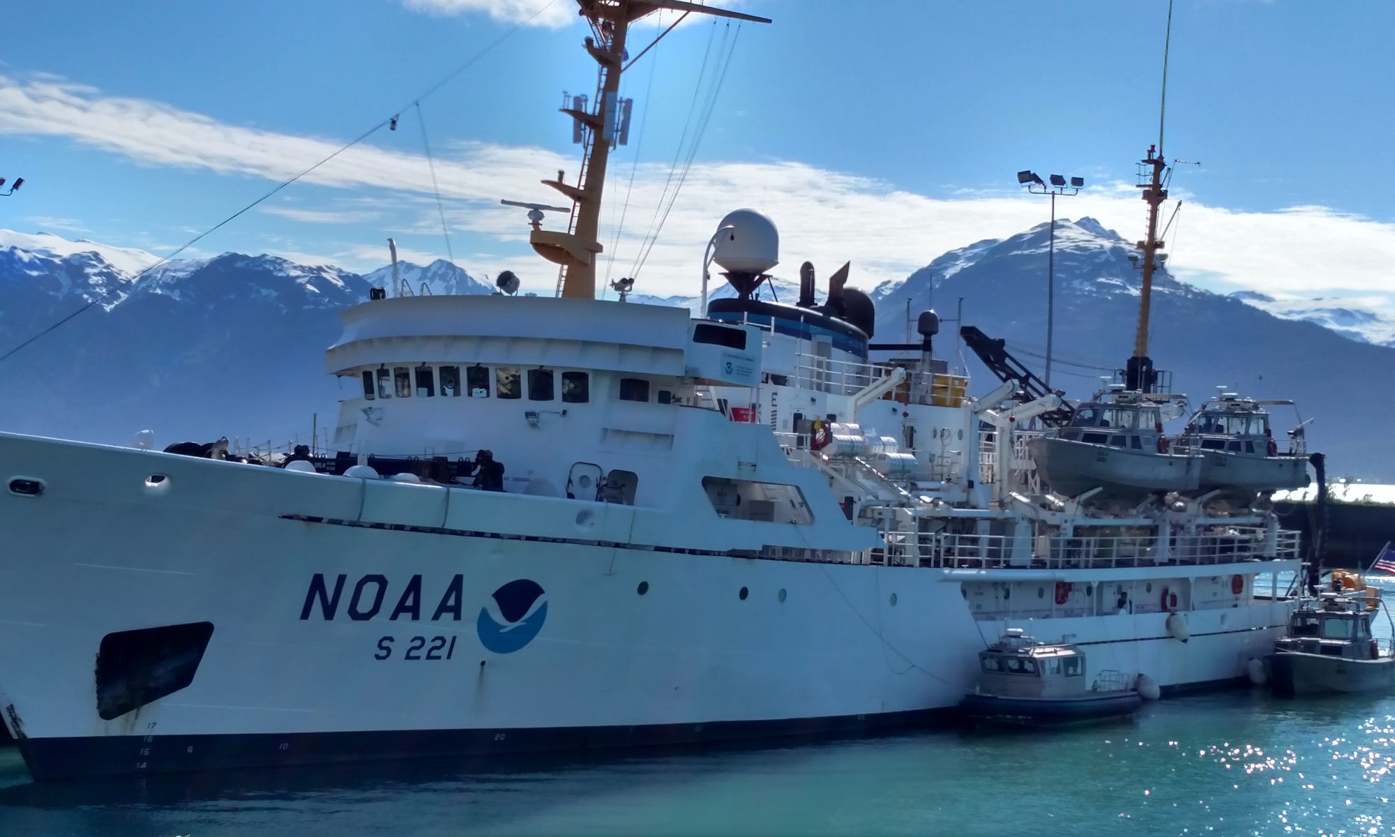
Onboard NOAA Ship McArthur II
June 4 – 9, 2007

Mission: Collecting Time Series of physical, chemical and biological data to document spatial and temporal pattern in the California Current System
Geographical Area: U.S. West Coast
Date: June 6, 2007

Weather from the Bridge
Visibility: clear
Wind direction: 291
Wind speed: 16 knots
Sea wave height: 2-3 ft.
Swell wave: 5-7ft.
Sea temperature: 14.671 C
Air temperature: 16.1 C
Sea level pressure: 1021
Cloud cover: 25% scattered cumulus

Science and Technology Log

Up at 07:00 Discussion continued on how to do deep casts with CTD and avoid kink in wire: lower it slower or put on more weight or etc. Some staff short on sleep after working with CTD repair last night. I do fine on six hours a night but I feel it when it’s five. I will try for a nap today.

Cast 13 and 14 were done with other staff and went without problems. They will try a deep cast again today.

Cast 15 08:00 Station 65-90 Latitude 35.03387N Longitude -127.45604 W at depth to 1000 m; CTD cylinders tripped at 1000, 200, 150, 100, 80, 60, 40, 30, 20, 10, 5, 0 meters In the wet lab work the funnel for sample #8 was not locked tightly and the apparatus leaked. I put on a new filter and took another seawater sample for #8. Samples processes and stored. Data for cast is Table 7 at the end of the report.

The two 4′ by 6′ incubators on deck contain the C14 spiked samples placed in a continually flowing seawater bath for twenty-four hours. Samples are placed in metal tubes with various numbers of holes in the tubes. The various tubes are designed so that the samples are exposed to 50%, 30%, 15%, 5% and 1%. One set of samples is not in tubes, but in full sunlight. Then they are evaluated for the rate the phytoplankton incorporate the Carbon 14 as described in Day 3.

Began chlorophyll analysis on the filtered specimens from the range of depths at each station that have been in the freezer more than twenty-four hours.

Marguerite went over the procedure using the flurometer to process the sample. It must be turned on at least one hour before running the tests and the chlorophyll samples #1-12 plus 1 and 5 micron samples must be at room temperature in the dark for at least one hour before beginning. She calibrated the flurometer with acetone. We rinse the cuvette three times with a couple of milliliters of sample, and then add the remainder to the cuvette. It will be about 2/3 full or more. Wipe the cuvette well with a lab wipe to remove any oil on glass from your hand/fingers, place sample gently into flurometer. The first reading should be taken after it has stabilized, usually 15-20 seconds. Then two drops of 5% hydrochloric acid are added to degrade the chlorophyll pigment. A second reading is taken to measure the remaining pigment. These are recorded on a “Bottle Sample Data Sheet”, an example of which is included as Table 8 at the end of the report. After measurements are recorded, the sample is thrown out in a collection container and the vials disposed of in a waste container.

The cuvette is rinsed three times with acetone and then begin processing the next sample. Again it really helped to have seen this procedure demonstrated on the DVD that was sent to me ahead of the trip. I was much better prepared. It was important for the research done as well because if one made a mistake in the sample procedure, there was no sample in reserve to be able to run the test again. I did samples for a couple of hours in the afternoon and a couple more in the evening when I was scheduled for working but waiting for a cast to come up.

Cast 16 and 17 were processed by other team.

Cast 18 @ 15:35 Station 67-90 Latitude 35.4670N Longitude -124.9409 W Cast depth 4380 went very well. Processed by Erich and Charlotte. Cylinders tripped at 4380 bottom, 4000, 3500, 3000, 2500, 2000, 1500, 1000, 750, 500, 250, 0 meters; Data for cast as Table 9 at the end of the report.

I observed a couple of bongo net tows today. Live net tows are collecting zooplankton and other seawater specimens from the first 200 meters of depth. The bongo nets have two .8-meter diameter rings with a mesh net and a polycarbonate tube at the end. The nets were deployed using the ship’s starboard winch equipped with at least 300 meters of wire. The ship maintains a vertical wire angle during the tow of approximately 45 degrees. Kit Clark, the oceanographer in charge of net tows said it was important that the winch be able to maintain a slow, constant retrieval speed. When nets are retrieved, they are hosed down to wash specimen sticking to the mesh down into the polycarbonate tube. The specimens are transferred to jars and fixed with formalin. There were a lot of krill and one viper eel in the specimens I observed this morning.

Wildlife observer saw three albatross today. Cast 19 @ 21:14 Station-NPS-8 Latitude 35.325665 N Longitude 124.438304 W Cast depth 1000 meters; Cylinders tripped at 1000, 900, 800, 700, 600, 500, 400, 300, 200, 100, 50, 0 meters; Nutrient samples only taken for this cast; Data for cast is Table 10 at the end of the report.

Cast 20 @ 11:29 Station 67-85 Latitude 35.6249 N Longitude -124.5544W Cast depth 1000 meters; CTD cylinders tripped at 1000, 200, 150, 100, 80, 60, 40, 30, 20, 10, 5, 0 meters; Bottle # 2 leaked, was empty, so no sample collected. Always check that funnels are locked tight before I begin. Samples processed and stored; Data for cast is Table 11 at the end of the report.

Long discussion of the structure and movement of ocean currents. Dr. Collins is a brilliant scientist, such depth in oceanography. He uses vocabulary during his explanations that need explanation in themselves. The Great Lakes and fresh water bodies are a lot simpler.

Discussed with Dr. Collins the military value of the studies we are doing. He said the military does sea floor mapping, looks for mines and things on the sea floor. He explained that there are levels of optimum transmission of sound, channels for submarines. Determining these best channels relates to the salinity and temperature

Bed @ 01:00 June 7th

June 5, 2007April 1, 2021

Elsa Stuber, June 5, 2007

NOAA Teacher at Sea
Elsa Stuber
Onboard NOAA Ship McArthur II
June 4 – 9, 2007

Weather from the Bridge
Visibility: Clear
Wind direction 275.64
Wind speed: 13 knots
Air temperature: 16.1 C
Sea wave Height: 1-2 feet
Seawater temperature: 13.98 C
Swell wave: 4-6 feet
Sea level pressure: 1017.4
Cloud cover: 50%, stratus

Science and Technology Log

Up at 06:00 and went to flying bridge to observe with Kathryn. Not much wildlife to see other than a few sea gulls. Color of water so blue. Temperature is cool early in the morning. Breakfast good fruit, lots of starches, sausages. A time to talk to crewmembers about the different trips of MCARTHUR II from Alaska to Peru. Jim spoke in detail @ working as a fisherman in Alaska, ice in his moustache, not needing very heavy clothes because you worked so hard you got hot. He said it was 06:00 until 22:00 in summer time. He spoke about fishing limit rules, coordinating with Japanese fishing boats, and also how the catch numbers have fallen since ten or fifteen years ago.

Cast 6 and 7 were early in the morning with other cruise staff. All proceeded as expected.

Cast 8 @ 08:18 Station 60-75 Latitude 37.067N Longitude 124.4145 W Cast depth to 1000m; CTD cylinders tripped at 1000, 200, 150, 100, 80, 60, 40, 30, 20, 10, 5, 0 meters Data for cast is Table 5 at end of report. Cast information time is always written in Greenwich time; I subtract seven hours to show our time on ship for the station work. The Cast information listing for latitude and longitude is close but not exact to Table 1 for the CalCOFI stations. In the 1000 meter depth casts it takes about forty minutes for the CTD to go down to depth and come up again, stopping at the different levels for the specific rosette to open.

I learned more information on the testing of samples from Marguerite Blum, MBARI oceanographer: The nutrient samples contain nitrates and nitrites as well as silicates, phosphates. The nitrates and nitrites area examined at Moss Landing lab with an auto flow analyzer, which translates sample into voltage and indicates the amount of the nutrient in the sample.

QP (quantitative phytoplankton) will show up to fifteen general types of phytoplankton in a sample. This is an expensive test to run. The flow cytometry test divides the sample into four groups: bacteria, prokaryotes, eukarotyes, and zooplankton. It will determine a general number of how many of each are present in the sample.

The Carbon 14 test shows the amount of carbon uptake by the phytoplankton. C14 of specimen fluoresces and radioactive emission level counted on a scintillation counter. The chlorophyll analysis of the green chlorophyll is run on the flurometer. Samples that have been in the freezer 24 hours we will process in the dry lab while on this cruise. On this cast I also handled the A* filter, the HPLC filter and the POC filter, placing them in their red, blue, and green cryovials respectively, and then put in the liquid nitrogen container. The analysis of HPLC, POC, FCM and N15 samples are not done at Moss Landing but are sent out to other labs for processing.

Cast 9 @ 11:45 Station 60-80 Latitude 36.5677N Longitude 125.0327 W Cast depth to 1000m; CTD cylinders tripped at 1000, 200, 150, 100, 80, 60, 40, 30, 20, 10, 5, 0 meters; Data for cast is Table 6 at end of report.

There have been bongo net tows at our stations, but often when I am working or sleeping. I have seen some of the specimens caught which are in jars with formalin. I hope to see a net tow start to finish soon.

I have watched with Kathryn, the Mammal observer, during different periods today and have not seen any wildlife. She saw seven dolphins earlier in the day. I asked her about the tagging of sea life and she talked about the guidelines. She said the organization had to apply for a permit to the National Marine Fisheries. This may take up to a year to obtain. A boat doing tagging must display a special flag with a research number on it. The permit will specify the number of “takes” (getting close to or affecting the animal such as a whale or turtle). She said a lot of information was available on line at TOPP (Tagging of Pacific Pelagics). When it’s on the surface, the signal from the tagged animal will beam up to satellite and transmit its location. How long it will function depends on the battery life, and of course a small animal can only carry a small battery. The scientist will set the frequency of the beam according to the frequency of the animal at the surface. A sea lion surfaces every fifteen minutes so its battery will last three weeks. A turtle will surface every second day so its battery will last six months to a year or more. Scientists want to recapture radio equipment so watch closely at the animal’s location. The equipment will give off a signal for at least a week after it falls off. Researchers put gummy worms under the suction cups on whales and know it will take about a week for that sugar to be dissolved, and then the apparatus will fall off. Tic Tacs with suction cups also work.. The equipment is numbered for location and will be returned if found by any ships, any countries at sea. She said a problem that can occur is that is that the sensor on the collar could get algae grown over it so it stays off.

Cast 10 and 11 were with other cruise staff.

Cast 12 was started @ 22:45 and was to be a deep cast, 4500m. When it reached @1100m transmission of data stopped. The CTD was brought back to the surface and worked on by staff about three hours. A kink had developed in the wire. That section was cut out and all connections redone.

Data retrieved gives information for the 1100 m at this location for beam transmission, salinity, temperature, and fluorescence all taken by the computer monitoring system in the dry lab. Bottle samples were not taken.

To bed @ 02:00 June 6th I am greatly stewing about the CTD problems with all it means to the research, to the cruise, and the expense of it all.

June 4, 2007April 1, 2021

Elsa Stuber, June 4, 2007

NOAA Teacher at Sea
Elsa Stuber
Onboard NOAA Ship McArthur II
June 4 – 9, 2007

Weather DAY 2: San Francisco to sea
Visibility: Some fog before 12:00, which later cleared
Wind direction: 282.14
Wind Speed: 9 knots
Sea wave height: 1 foot
Seawater temperature: 14.159 C.
Sea level pressure: 1017.15
Air temperature: 14.1 C
Cloud cover: 100% stratus

Science and Technology Log

Awoke 06:00 and did journal work until 07:15 breakfast. Studied cruise information. As suggested by CS Tim, I took a Dramamine II last evening and one this morning. I don’t want to have seasick problems. I don’t feel any side effects from the medication.

Safety meeting 09:00 with FOO Middlemiss. It is important to close the heavy doors when going and coming on the ship. We reviewed procedures for Man Overboard, Fire, and Abandon Ship.

Fire: signal = 10-second continuous bringing of the General Alarm bell and a 10-second continuous sounding of the ship’s whistle. Proceed to fantail of ship.

Abandon ship: signal =seven or more short blasts on the ship’s whistle followed by one long blast. Bring survival clothing and PFD to life raft location on the bridge. We practiced putting on survival clothing: feet and legs in then hood on your head before putting arms in sleeves and zipping up. Difficult to do getting arms in by yourself; this is not a quick maneuver. Mine was the smallest size; feet and arm-hand portion pretty big on me, but I would survive. I brought my mustang survival jacket along on the cruise as well.

Man Overboard: If witnessed throw life ring buoy into the water and call for assistance immediately. After one minute throw a second life ring buoy in the water. Try to keep visual surveillance of the person in the water. Signal = three short blasts on the ship’s whistle.

For safety drills, dismissal from drill signal = three shorts blasts on the ship’s whistle. Mess hall information, store information, medicine location given.

Ship departed San Francisco approximately 10:15 with very foggy weather, foghorn blowing. It is very loud. If wearing plugs, the hearing of anyone working close to foghorn such as the wildlife observer on the flying bridge would be affected over time. Special ear protection is needed for persons at that observational post. Kathryn Whitaker is the wildlife observer on this cruise. She is stationed on the bridge with a lap top computer to record type and quantity of all birds and sea life she observes. Kathryn is observing from daylight to sundown except going down for meals. She uses powerful binoculars and camera to photograph whatever she sees. On some cruises she has two or more staff working with her, one of whom is typing in the computer all that the observers are calling out that they are seeing which is often a great deal if the ship is nearer shore than we will be for most of this cruise. As we leave SF Bay we see a dead gray whale floating, Kathryn points out the grease trail from the decaying whale blubber floating out on the water. There are cormorants and seagulls in large numbers flying in the area of the ship for the first three and a half hours of our trip. Then we only observe some seagulls.

The overall survey plan is to proceed offshore along CalCOFI (California Cooperative Oceanic Fisheries Investigation) Line 60, occupying stations each 10-20 nMi (nautical miles) to ~175 nMi offshore. Then proceed to stations each 20nMi northeast to station 67-90 at the offshore terminus of Line 67, and work back into shore along Line 67 with stations 10-20 nMi apart. After the station work is completed, the ship will return to San Francisco and offload gear and personnel. I will include the CalCOGI station information in Table 1 and Figure 1 of this report.

Operations at the stations are to collect physical, chemical, and biological data by CTD (conductivity, temperature, depth) and its rosette bottles, net tows, and underway surface measurements. All CTD casts at the stations are to the bottom or 1000 dbars whichever is shallowest. At stations #12 and #16 two deep casts (4500m) are planned conditions and time permitting. Secchi disk cast will be made at daytime stations. HyperPro optical sensor casts are to be made at midday stations. Oblique bongo net tows will be to 200m depths.

CalCOFI survey continuous operations while underway will include logging meteorological and sea surface property, a pCO2 measuring system in the wet lab, the incubators for chlorophyll seawater samples on the fantail, and the marine mammal observer.

Cast 1 @ 13:51 Station 60-50, Latitude 37.948N & Longitude -122.888W, Cast depth 40m, Bottom depth 48m, CTD cylinders tripped at 40, 30, 20, 10, 5, 1.5, 0 meters Data for cast is Table 2 and accompanying data graph including percent beam transmission, depth, temperature, and fluorescence at end of my report. Participants: Tim and Erich from MBARI, USN Charlotte, TAS Elsa This was good hands on practice for the sampling work. Charlotte and I received a lot of help, tips for technique. Tim is very patient with our learning curve.

We check stopper at bottom of rosette cylinder to determine that it didn’t leak. Pull out stopper and should only be a couple of milliliters squirting out. Then open valve at top of rosette to take the sample.
Open stopper by lining up black circle drawn on stopper with peg on stopper and pull out. Rinse 280ml sample bottle three times with @ 15ml of sea water from rosette and then fill sample bottle to overflowing, close stopper. Rinse small nutrient sample bottle 3 times and then fill it half to two-thirds full. Tim and Erich were filling other bottles for C14, N15, POC, QP, HPLC, FCM, and A* tests which are described below.
In wet lab, nutrients numbered sequentially are put in cartons and then promptly put into the freezer. These will be processed later at the MBARI lab.
Funnels with filters for the twelve samples were set up prior to reaching the station. Turn on aspirator pump. Filter solutions through flasks. Suction for all samples is improved if you turn off valve on those that have already filtered through. You can’t get paper filter off the filter piece if suction is still operating. Be careful at all times to check that sample number matches its numbered filter apparatus, and glass vial the filter is stored in when filtration complete.
Put particular filter for the fractionated 5 micron and 1 micron filtering. Sample is labeled “F” collected by MBARI scientist. Pour 100ml of sample into each funnel for these samples.
Add the 10ml. measured amount of 90% acetone to each glass vial with its filter to “fix” the phytoplankton on the filter. Place these in the carton in sequential order to be placed in the freezer. These remain there in the dark for at least 24 hours before we can test for chlorophyll levels with the flurometer.
Label samples for casts read for example S307c#2, #5. Meaning June 3-9 Cruise S307 cast #2 sample #5
Three other filtrations were done which are color labeled: green POC organic carbon, how much carbon is in the water other than the plankton detritus; red A* filter will be evaluated in spectrophotometer to get all wave lengths of life, not just chlorophyll; and blue, HPLC -high performance liquid chromatography which will show 23 pigment types commonly associated with different algae so they may be qualified and quantified for the level the sample was taken.
The MBARI scientists take the C14 and N15 radioactive samples.
Set empty bottles in rack and carrying case and put out on back deck to be ready for the next cast. Put new filters in the 12 funnels in the wet lab to be ready for the next cast.

Chief Scientist Tim Pennington sent a DVD with demonstrations on how different sampling and testing of the samples are handled. It was very helpful to see this walk through ahead, with emphasis on the problems that can arise with the techniques and suggestions on what to do about them.

Cast 2 @ 15:35 Station 60-52.5 , Latitude 37.864N Longitude -123.065W, Cast depth to 80m, bottom depth 90m; CTD cylinders tripped at 80, 60, 40, 30, 20, 10, 5, 0 meters Data for cast is Table 3 and accompanying data graph at end of report.

CTD goes down and is monitored by observer in dry lab, CTD technician Doug or Dr. Collins. The observer communicates with the bridge and crew to raise the CTD, stop at each specified depth, and to trip open the particular rosette flask at this depth.

I worked on Cast 2 and became a little more efficient. I’m continuing to try to observe all very carefully so as not to make any mistakes. Procedures are very precise for accuracy.

Casts 3, 4 were not on my watch. During that time I went to the flying bridge to do wildlife observation with Kathryn. There were numbers of cormorants and seagulls. She had seen four dolphins @ half a mile away earlier in the day.

Cast 5 at station 60-57.5 at 21:42 Latitude 36.86N Longitude -123.3612W Cast depth to 1000m; CTD cylinders tripped at 1000, 200, 150, 100, 80 ,60, 40, 30, 20, 10, 5, 0 meters Data for cast is Table 4 and accompanying graph at end of report. The water from 1000 meters is very cold, 3.843 C compared to 12.144 C at the surface.

The seas are pretty calm so collecting water samples, working with the equipment, walking around is not a problem. I have no hint of seasickness so I won’t continue to take Dramamine unless I begin to feel queasy.

Spigot on rosette #12 black circle marker has faded and needs to be remarked.

Go to bed @ 00.30 6/5/07. I’m sharing quarters with three others and my bed is a top bunk. Bunks are not very big, but I’m only 5′ tall so size of bunk is not a problem. I can just barely sit up though and it is tricky to make it up in the morning. Plenty of blankets and linens supplied.

June 3, 2007April 1, 2021

Elsa Stuber, June 3, 2007

NOAA Teacher at Sea
Elsa Stuber
Onboard NOAA Ship McArthur II
June 4 – 9, 2007

Weather DAY 1: San Francisco, Pier 30/32
Visibility: 10 nautical miles
Wind direction: 270 NW
Wind Speed: 8 knots
Sea wave height in harbor: 1′
Seawater temperature: 15.129 C.
Sea level pressure: 1016.4
Air temperature: 15.2
Cloud cover: 1/4 cumulus

Science and Technology Log

The day began @ 07:30 picking up equipment at Moss Landing and riding up to San Francisco in van with other MCARTHUR II cruise members: Chief Scientist Tim Pennington, Biological Oceanographers-Marguerite Blum, Kit Clark, Erich Rienecker, Troy Benbow, Charlotte Hill; Physical Oceanographer, Dr. Curt Collins; CTD technician, Doug Conlin. At Pier 30/32, Marine Mammal Biologist, Katherine Whitaker, joined us and the other Teacher at Sea participant, Turtle Haste.

Tim Pennington coordinated the staging operation with the (FOO) Field Operation Officer Lt. Amanda Middlemiss. The large equipment for the cruise was at the pier on a flat bed truck and was loaded by crane on the ship’s deck with the assistance of the ship’s crew. All scientists were involved in unpacking the gear and setting up the wet lab and dry lab for the Time Series study work. As these labs have been physically updated since the last MBARI cruise on MCARTHUR II, set up in these labs required some modifications. All staff commented on the benefits and advantages of the lab improvements.

I reviewed material I researched on line prior to cruise about the Monterey Bay Aquarium Research Institute (MBARI) Time Series program. The focus is on the relations between oceanic carbon and nitrogen cycles and climate variability with emphasis on measuring the primary phytoplankton production. The research involves both observational and experimental studies with shipboard measurements of physical, chemical and biological parameters during cruises in Monterey Bay (since 1989) and offshore into the California Current (since 1997) at different seasons of the year. The data collected over this time span is being used to construct synthetic views of the oceanographic system dynamics of the California Current. The work has documented seasonal cycles, El Ninos and La Ninas and longer decade-scale cycles (e.g., Pacific Decadal Oscillation). The overall goal is to learn as much as possible about the earth’s climate and ocean systems, and therefore it is important to understand these cycles. Beyond construction of views of the California Current cycles and understanding the causation of them, will scientists determine that the directions show potential effects of global warming?

As stated in the summary of the MBARI Time Series Program report 2007: “Is this a local-or remotely-driven effect? We are uncertain. Is it important? You bet. Why? Because we area certain that (1) conclusions about global climate change begin with local observations, and (2) unusual conditions are often highly informative.”

Chief Scientist (CS) Tim Pennington went over the wet lab organization with the three of us new to working there, defining the different sample bottles and chemicals used in collecting and processing the sea water samples. He showed us which type of samples were stored in the freezer or in the liquid nitrogen, and which were placed in the seawater bath on the back deck. We signed up for our individual research tasks, my assignment is seawater sample collection from the rosette bottles of the CTD and processing in the wet lab. When filtered samples are ready, to process with the flurometer for chlorophyll level. My shift is 08:00 – 12:00 and 20:00-24:00. I work with CS Tim. Then we are free to study/work in other areas as you would like or as you are needed. We put duct tape ridge along front edge of wet lab tables to help stop materials from sliding off counter if ship is rolling.

At 16:00 we moved our personal belongings to our assigned quarters and then were free to explore the set-up of the MCARTHUR II. Important to note were the areas where one must wear a hard hat and a PFD. No open toed footwear outside your quarters. Pay attention to stay far away from winches when they are being used.

FOO Lt. Middlemiss requested that we review the safety instructions packet found in our quarters and that we should be ready for the safety drill to take place the next day.

Bed at 00:30 June 4th.

October 11, 2006April 1, 2021

Scott Dickison, September 30-October 11, 2006

NOAA Teacher at Sea
Scott Dickinson
Onboard Research Vessel Shearwater
September 30 – October 11, 2006

Mission: Quantitative Finfish Abundance
Geographical Area: Channel Islands Marine Protected Areas
Date: September 30 – October 11, 2006

Prologue

The cruise that I participated on was a multi-part project that spanned several weeks. I came on board for the final, and most interesting part of the project. Those parts you can read about in my log entries, however some background and technical information may be useful to better understand the operation.

The cruise took place onboard the NOAA R/V Shearwater. The project was called a Quantitative Finfish Abundance and Exploration of the Channel Islands Marine Protected Areas. A cooperative Remotely Operated Vehicle (ROV) study with the California Department of Fish and Game, Marine Applied Research and Exploration, and the Channel Islands National Marine Sanctuary.

When I arrived, the bulk of the work had been completed and it was time for the experimental portions of the project to take place. These experiments were designed to ensure the reliability, precision, and accuracy of the quantitative data collected by ROV survey. The basic operations involved live boating the ROV along predetermined track lines. That is, the RV Shearwater would proceed along a predetermined line on the surface that the ROV was also independently operating on at the ocean floor. The ROV had a range of 50 meters from the stern of the RV Shearwater. The ROV pilot had on-screen-display (OSD) from the video cameras mounted on the ROV, as well as an OSD that displayed the ROV position relative to the mother ship. This display is generated with the use of a sonar beacon mounted on the ROV and a sonar receiver lowered over the side of the mother ship.

On to the logs…

Saturday 9/30

Arrive at the R/V Shearwater. Got the lay of the land.

Sunday 10/1

Head out of the Santa Barbara Harbor in transit to Santa Cruz Island to pick up the research crew. With the team of scientists on board, we head out for our destination of East Point on Santa Rosa Island for the first deployment of the ROV.

The weather turned on us, with the winds blowing and the rain pounding. The seas got rough and the going was slow. This being the first day out, the sea legs had yet to be adjusted. This was the cause for a quick retreat to the head…

Finally made it to our testing location. Weather was dismal as the ROV was launched. Today’s mission was to “paint” fish with lasers mounted along side the ROV camera. This was a very interesting procedure designed to measure fish length. Essentially capturing a fish on video and “painting” it with two laser dots at the known distance of 11 cm. Total fish length can then be calculated either by determining fish camera fish length and laser dot space, or by using the screen width and the fish length in comparison.

This day I became umbilical tender and hydraulic operator for launching and retrieving the ROV. I also observed the underwater video and fish painting process. This was a very interesting day becoming part of the crew and assisting in the work. Due to a couple of technical issues, we returned to Santa Barbara for the night.

Monday 10/2

While crewmembers were working on correcting the technical issues, I assisted others with setting up lines for the next set of experiments. This required setting up vinyl covered steel cables at a length of 110 meters and marking them with colored flags every 10 meters that would be easy to view through the ROV cameras. These cables were also set up with loops on each end for linking together, or for securing weights. The cables were then spooled for ease of deployment and stowed for later use.

The technical issues as well were repaired and again we set out to sea. This day’s destination was Anacapa Island. With some sonar scanning, a sight was selected for the next sets of experiments, to determine accuracy of transect distance precision across the spatial dimension.

For this experiment, the 110 meter cables were laid across the bottom with high relief profiles. This distance of cable would provide a length of 100 meters to run with the ROV. Divers also swam the line and took depth readings along the cable. The cable ran up and down over rocks and various substrates that are considered fish habitat. The concept being that there were more lineal feet of fish habitat in this relief than straight line distance. The ROV recorded this distance, but this was a means to determine if those recordings were an accurate measurement.

The sight we were working was spectacular. We were on the southern tip of Anacapa Island. The shoreline of the island was shear rocky cliffs. The cliffs are a major nesting and roosting sight for the endangered California Brown Pelicans, they were everywhere both on the cliffs and circling in the sky. The area was also populated with sea lions. They were very amusing swimming around the boat and with their barks echoing off the cliffs of the island. After the work here was done, we headed north for a protected cove to drop anchor for the night.

Brown pelican nesting area on the high cliffs

Tuesday 10/3

This day we headed back toward Anacapa to continue the track line experiments. Another shallow depth sight was selected toward the North end of the island. The same procedures were used here laying out the cable lengths that were then checked by divers and then run with the ROV.

The water was thick with small baitfish that was being fed on by schools of Bonita. This was a sight to see, and was particularly amusing to see the pelicans dive-bombing into the water also feeding on the baitfish. This went on for most of the day. Operations went well today and when complete the gear was collected and stowed. We headed off to another protected cove for the nights anchorage.

Wednesday 10/4

We continued the track line experiments today. Work was going well so we started preparations for the next upcoming experiment. The preparations consisted of setting up fish models of various sizes and securing weights to then to enable deployment of them floating various heights off the bottom. The fish models were constructed of a flat piece of neoprene with color copied pictures of the local significant fish species laminated and attached to the sides.

The sight of the day was a pod of dolphins leaping out of the water and splashing around in some sort of frenzy. We assumed the must have been feeding, but were not really close enough to tell exactly what was going on. Today’s tasks went well and I went out on the Avon to retrieve the cables and the divers. With all back onboard, we headed off to the nights anchorage.

Thursday 10/5

Today we set out for a deep water site to continue the track line experiment. The previous sites had been in the 10 to 20 meter depth zones. Today we would run the track line experiment in a 50 meter depth zone. This posed a different set of circumstances. The tracking cable was spooled into a basket for deployment. It was then deployed skillfully and precisely by the well experienced deck officer. With the cable in place, the ROV was launched to run the line. This depth was to deep to send divers down, so the ROV did all the work. Tracking went well and the ROV was brought back on board.

Recovery of the gear was a bit more difficult. We had to haul back the cable and weights with a power winch as opposed to winding it back by hand in shallow water. After we got about half of the length back, it got jammed and snapped so fast my head spun. At least the experiment was completed.

After gathering and comparing the ROV data with the diver collected data it was apparent that the ROV collected nearly identical data to the diver collected data. This experiment seemed to be a success. ROV use and procedures seemed to be a reliable means to determine transect distance across the spatial dimension by my observations. Naturally the collected data would be reviewed later by the scientists on board to accurately determine the results.

During the day we continued to prepare the fish models for deployment tonight. With the track line experiments complete, we headed for a location suitable for the fish model experiment. This experiment was conducted in the evening to simulate the light conditions in the typical habitat depth of 50 meters. The point of the experiment was to determine the accuracy of fish length as determined by ROV survey. The ROV survey used both paired lasers and distance sonar to determine fish length. When these procedures are utilized on fish models of known length, the scientists could determine if the process could be accurate when video capturing wild fish in the test zone.

As we arrived at the experiment location, the sun was setting and a most beautiful full moon was rising over a distant horizon. Divers were used to strategically deploy the models to simulate populations of wild fish. The ROV was deployed and ran the line of fish models while video capturing the images. Tonight I had an opportunity to pilot the ROV. I thoroughly enjoyed this opportunity and spent some time observing some flat fish scurrying about the bottom as I waited for the divers to collect the fish models. Soon all was complete, the divers came back on board, and we recovered the ROV safely. We remained at this location for the night, it was quite beautiful.

Friday 10/6…the final day.

Today was a public relations day. We returned to Anacapa and met up with the California Dept. of Fish and Game boat, the R/V Garibaldi. They had brought some local writers and reporters out to cover the project. We still went on with the normal operations of surveying fish populations. It was another great day on board the NOAA R/V Shearwater as a participant in the Teacher at Sea Program! Back to Santa Barbara we cruised.