echogram – NOAA Teacher at Sea Blog

July 31, 2026July 31, 2026

Jo Slavitz: A Lot of Fish in the Sea: July 26, 2026

NOAA Teacher at Sea

Jo Slavitz

Aboard NOAA Ship Oscar Dyson

July 19 – August 10, 2026

Mission: Summer Pollock Acoustic Survey, Leg 3

Geographic Area of Cruise: Bering Sea, Alaska

Date: July 24, 2026

Weather Data from Bering Sea

Latitude: 58° 48.960’ N

Longitude: 173° 43.168′ W

Winds: E at 15-20 mph

Air Temperature: 45.68° F (7.6° C)

“The charm of fishing is that it is the pursuit of what is elusive but attainable, a perpetual series of occasions for hope.” – John Buchan

Science and Technology Log

As the saying goes “there are lots of other fish in the sea,” so how exactly does NOAA Ship Oscar Dyson find mostly Alaskan pollock in such a huge ocean? It’s a combination of structured transect planning, analyzing complex acoustic data and a little bit of luck.

Transects: At first glance the map of the 3 legs of the Alaskan Pollock Survey look like a crazy zig-zag path, so what’s going on and where are we going? The Oscar Dyson is traveling on a transect. A transect is a line drawn by scientists across an area used to measure, count and record the species living there. Oscar Dyson scientists are tasked with figuring out how many pollock are living in the Bering Sea, what age they are and their reproductive stage. As Oscar Dyson travels along each transect, the scientists decide where good places are to sample the pollock population using a long trawl net. It’s difficult to look into the ocean (though we will talk about cameras later) so NOAA scientists actually “listen” for the fish as they swim under the boat.

line drawing of NOAA Ship Oscar Dyson demonstrating acoustic calibration. we can see the sounding board extending beneath the hull; metal calibration balls are suspended farther beneath the sounding board. — The sounding board on the bottom of Oscar Dyson sends and receives frequency information. (NOAA Fisheries)

EchoSound: Many people are familiar with the way animals such as bats and dolphins emit sounds and use echoes to gather information about their surrounding environment. The scientists on the Oscar Dyson also use sound and echoes to gather information about their environment in the Bering Sea. The boat has a sounding board underneath called a transducer that emits energy pulses at different frequencies and receives the echoes as they are bounced back. Objects with different densities send back different amounts of echo energy. Scientists in the Acoustic Lab onboard Oscar Dyson watch a screen for echo patterns that match the patterns that are expected from individuals and schools of pollock.

photo of a screen displaying an echogram. in this graph, the x-axis is time and the y-axis is depth; colored dots represent the intensity of backscatter from a particular frequency encountered at each depth over time. — An echogram is a visualization of an echosound

Check out this image of an echogram. Echograms are a visualization of detected echo sounds. The bright red lines at the top and the bottom of the screen represent the surface and the dense ocean floor. The top wave of blues and greens is referred to as the “munge” ; it is a mixture of stirred up air bubbles, algae, plankton and other things that the team has determined is not pollock. Pollock are primarily in the area just above the bottom to about the middle of the water column. Boney fish such as pollock have a specialized organ called a swim bladder which allows them to take in and release gas, thus changing their density and allowing them to rise and fall in depth like a submarine. Not only is this organ useful to the fish, the air it contains has a different density from the surrounding water and reflects the echo energy that is emitted and picked back up by the ship’s transducer. Look carefully and you can see little colored dots and patches just above the ocean bottom depicted on the echogram. Those are fish and schools of fish. The scientists are confident that they are pollock but to be sure they need to collect a sample of the fish in those areas and get measurements from them.

diagram of a trawl net being pulled behind a vessel. labels point out the codend (the narrowest part at the back); the headline rope; the sweeps (lower lines); the weights attached to the lines; warp wires connecting the trawl to the vessel; and otterboards to help direct fish into the net. — Basic Trawl Net (source: Nettingland.com)

Trawl: Once a spot has been identified by the scientists, a call goes out to the crew, “Fishing, Fishing, Fishing”. This alerts all aboard that the vessel is going to break from the transect and drop the nets into the spots that had lit up with fish patterns on the echogram. The net is rolled out from a giant spool controlled by the deck crew rather than the scientists. The tip of the net is called the codend, from the old English word “cod” meaning a bag or pouch and this is where the fish are collected. At the opposite end of the net is the opening where fish enter. The weave, or meshes, of the net gets progressively tighter the closer it is to the codend.

three crewmembers wearing hard hats and life vests kneel to attach equipment to a portion of the trawl net on the deck of NOAA Ship Oscar Dyson — “Turtle” being attached to the kite

photo of the output from the FS70 echoscan showing a radar image across two-thirds of a circle — “Turtle” being attached to the kite

Attached to the net are several pieces of equipment that allow the scientist to analyze what is going into the net and when, during the trawl. The FS70, or netsounder, is a bright yellow device that also uses echoes to gather information. This piece is also sometimes called the “turtle.” You can see the crew here connecting it to a special part of the net called the kite. The kite and netsounder are attached and fly just above the opening of the net allowing the scientist to monitor what is going in.

Next to the picture of the crew you can see the image of what is being recorded by the netsounder on an information panel. This image of the “turtle” shows whether it is flying correctly, or oriented in the correct direction. The 2/3 circle image is a visualization of the echos the netsounder is receiving. The rainbow of color on the very bottom of this circle is the echo bouncing back from the bottom of the ocean, above that is another rainbow that represents the bottom of the net, above that if you look closely there are small blue marks just forming an oval with the rainbowed net bottom, those are the top of the net. When fish go into the net, they are represented as small dots, or blobs if a whole school is captured within this oval. The screen showing the echogram from below the ship and the screen with the netscan are placed next to each other on the control panel so that scientists can see the fish coming and hopefully adjust the nets accordingly to catch them.

close up view of a control panel showing two displays: the FS70 echoscan output, and the echogram of acoustic backscatter. — The control panel on the Bridge.

Scientists only want a sample of the fish, so they monitor the netsounder until they feel they have enough fish to accurately represent what they are seeing and then call “Haul Back.” This call tells the crew to raise the net back onto the boat, and the science crew to put on their wetlab gear in preparation for fish processing.

Try It on Dry Land

Swim bladders allow fish to change the density and buoyancy of their bodies, allowing them to change their position in the water column. Buoyancy is an upward force of an object causing it to float or sink. You can make a simple model of a fish’s swim bladder (and a fun catch game) using items found around your house.

You need:

Paperclips
1 pen cap (Bic pen or other with the stick part)
1 soda bottle with cap
Clay

Instructions:

illustration of a hand holding a plastic bottle filled with water and the pencap diver — Source: sciencebob.com

Fill bottle to top with water
Secure clay around stick of pen cap (do not cover opening)
Bend paperclip to form hook
Attach paperclip into clay with hook pointing down
Drop cap/hook into soda bottle so that it floats
Twist another paperclip into an L shape and drop to bottom
Put cap tightly on bottle

To Activate:

Squeeze the bottle and watch the pen cap drop
Release your grip and pen can will rise
Practice controlling where in the water column you can direct the cap
Can you dive the cap to the bottom and hook on to the L shaped paperclip?

What in the Science is going on… The cap holds a bubble of air underneath which allows it to float. When you squeeze the bottle the pressure makes the bubble smaller and changes the density of the cap causing it to sink. A fish’s swim bladder works by the same principles. Find out more here: www.instructables.com/Cartesian-Divers/

Personal Log

a circle, representing the earth tilted on its axis. arrows point out the north and south celestial poles, the meridian, the zenith (90 degrees). ellipses inside the circle represent three different paths of the sun. the first, closest to the north celestial pole, is labeled "Sun's path on July 21." The middle one, around the celestial equator, is labeled "Sun's path on March 21 and Sept 21." The third, closer to the south celestial pole, is labeled "Sun's path on Dec 21." — Sun Path Diagram

Life on Oscar Dyson is different in many ways then life on land. For one, the scientists work in shifts. There is a 4 am to 4 pm shift considered the dayshift and another from 4 pm to 4 am considered the nightshift. Acoustic monitoring and fishing happen all day and all night. I am on the day shift. Adding to the change in daily rhythms is the extended amount of daylight during the Alaskan summer season. The sun is up and bright when I hit my bunk to sleep. The sun will not set until approximately 12:30am, some nights I have gotten up in the night to watch the sunset out my window. I report to the Acoustic Lab at 4 am in the dark to find out what the night shift has been working on, the sun will then rise again at around 7 am. It takes some getting used to as the sun is a natural trigger for my body to know when to be active and when to rest. It makes for a long day, but who can complain with such a stunning beginning.

a beautiful view of sunrise over railing of the ship. there is a pile of rope in the foreground. the sky is golden, and the water, curling softly with the ship's wake, reflects the gold light. — Bering Sea Sunrise

July 7, 2026July 16, 2026

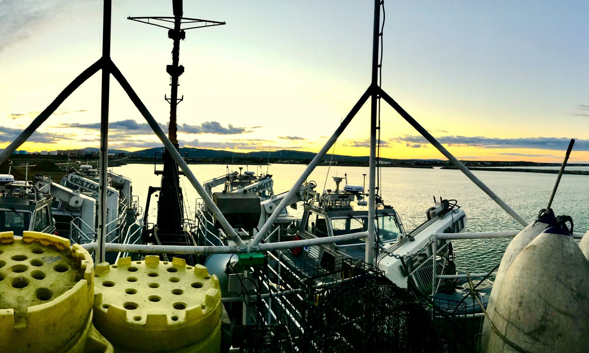
Guy Sturdevant: The Cave part 2, July 6, 2026

NOAA Teacher at Sea

Guy Sturdevant

Aboard Oscar Dyson

June 21 – July 15, 2026

Mission: Summer Pollock Acoustic Survey, Leg 2

Geographic Area of Cruise: Bering Sea, Alaska

Date: July 6, 2026

Weather Data from the Bridge

N 59.52° W 172.60 °, 0 AMSL

Conditions: Overcast, Seas at < 1’

Visibility: >5 NM

Wind: 90°/ 5 kt

Barometric Pressure 1016.1 mBar

Dry Bulb Temp: 45.3 ° F

Science Log

In my last post, we left off our acoustics 101 with the emergence of the first modern echosounders in the 1990s. Today, we will look at the current system aboard Oscar Dyson and learn how the science team can use their knowledge of acoustics to estimate fish populations. First, let’s look at the physical components that make up the EK80 echosounder system.

the EK80 echosounder system, which looks like a stack of black computer housings with cables sticking out of them — *Each frequency requires its own transceiver. These six transceivers are the heart of the EK80 echosounder.*

Transceiver – a combination of a transmitter and a receiver; in other words, it both produces an electrical pulse to be sent to the transducer and converts the backscattered signal into usable data a computer can understand. You can think of the transceiver as the electronic brain that manages all of the signal inputs and outputs.

Transducer – Just like you might plug a microphone into your laptop to record audio, each transceiver needs a transducer to first convert the electrical pulse into an acoustic pulse that is transmitted into the water, and to measure the acoustic backscatter that returns. You can actually see the transducers in the photo of the centerboard below. The transceivers measure frequencies ranging from 18 kHz (those really annoying mosquito ringtones that only young people can hear are around 18 kHz) to 330 kHz.

close-up view of a center board - normally mounted beneath the ship, but currently hoisted up in the air attached to some sort of crane. an arrow points out red circles at the base of the centerboard, identifying these as transducers

The red circles on the bottom of the centerboard are the faces of the transducers. These sensitive instruments are mounted at the lowest point of the ship to isolate them from the vessel’s noisy hull. (Photo credit: NOAA)

The Echogram

Once the transceivers process the acoustic backscatter, the data is displayed on a screen for interpretation.

screenshot of acoustic backscatter readings, represented as a color-coded dots, across several panels. a superimposed text box identifies the depth as 109.5 m. — There’s quite a lot going on here! Let’s break it down into smaller pieces so we can learn to look at the data like a scientist.

the previous image of acoustic backscatter readings is repeated here, now with annotation. six vertical panels are identified with different frequencies: 18 kilohertz, 38 kilohertz, 70, 120, 200, 330. along the base of these panels, Guy has added a two arrow ranging from "bigger reflectors" to the left to "smaller reflectors" to the right. An illustration of a cod is at the "bigger reflectors" end of the scale, while krill and copepods appear toward the right side of the range. on the left side of the backscatter panels, there are now a few words along the y-axis, identifying the Surface of the water; the "Munge" (using the mock up album cover) just beneath the surface, Fish question mark in the middle of the water column, and seabed. — Each of the six frequencies appears as a vertical section that scrolls from right to left as the vessel moves. The top of each plot represents the ocean surface, and the thick red layer near the bottom shows the seafloor. The space in between lets us look at what is below the ship! Weak backscatter appears blue; stronger backscatter appears yellow and even red.

Our old friend munge is making an appearance in this echogram! It is the heavy backscatter layer just beneath the surface that is strongest at 18 kHz. Lower in the water column, we see that most backscatter occurs at higher frequencies, with only sparse backscatter in the lower-frequency plots. Backscatter that is observed only at higher frequencies indicates smaller organisms, such as krill or copepods. Backscatter that appears across all frequencies is likely generated by fish.

As you spend more time looking at this scrolling echogram, you can begin to recognize patterns and draw reasonable inferences. Below are some examples of the variety you can see in just a few hours in the cave.

a close up view of three panels (three frequencies) of an acoustic backscatter plot, or echogram. an arrow points to a thin vertical patch of red to identify it as "probable schools of juvenile pollock" — *Younger pollock can gather in schools 20-40 meters tall that appear as very thin red ellipses.*

close-up view of panels of an echogram showing acoustic backscatter readings. an arrow points to blue dots in the 18 kilohertz panel and identifies them as possible dispersed adult pollock. — You can clearly see occasional reflectors on the 18 & 38 kHz channels; these may well correspond to adult fish. The only way to be certain is to trawl in an area that looks like this and see what the net brings up!

example of an echogram (acoustic backscatter plot) with very little shading and few dots. it is labeled "Nobody is home." — *We know that large fish like pollock return a relatively even acoustic signal across every channel that we look at; there do not appear to be any significant pelagic fish present in this echogram.*

Now that we can read echograms, we are ready to call for our first trawl! Come back next time to see what we data we can scoop up in “The Anatomy of a Midwater Trawl”.

Personal Log

Things aboard Oscar Dyson have settled into a routine. We travel along acoustic transects during daylight hours, stopping 2-3 times a day to do a midwater trawl. Routine doesn’t mean boring, though! Maintaining a ship of this size and complexity is more than enough to keep everyone busy. The checklist for this leg included checking on the smaller craft that service and support Oscar Dyson on her mission. Conditions cleared on 06/29, and the Peggy D, the workboat that lives on the starboard hero deck, was given a thorough check and taken for a 30-minute voyage.

a small boat with a blue hull attached to the deck of NOAA Ship Oscar Dyson, in part by cables extending from davit arms. — *Peggy D secured to the aft hero deck of Oscar Dyson.*

a man and a woman in float coats and hard hats pose for a photo against the railing of the small boat as it churns away from NOAA Ship Oscar Dyson, visible on the horizon — *Peggy D secured to the aft hero deck of Oscar Dyson.*

Guy, wearing a life vest and neon green hard hat, takes a selfie on the small boat. we can see a woman in a float coat and hard hat sitting or crouching in the background, and a third person at the helm in the small boat's cabin. — *LCDR LeeAnn Keener and I enjoying the scenery.*

inside the small boat's cabin, Guy sits at the helm and another crewmember looks on. they both wear life vests and hard hats. — *LCDR LeeAnn Keener and I enjoying the scenery.*

first of three similar images: a person in a float coat and hard hat reaches a pole over the side of the small boat in motion

second of three similar images: a person in a float coat and hard hat reaches a pole over the side of the small boat in motion as a life preserver comes into view

Safety drills and practice are a part of the routine as well. ENGR Connor Rauch practices recovery during a man-overboard drill on Peggy D. In the case of an actual man overboard, the smaller vessels are used for recovery, as they can respond much more nimbly and are far safer in close quarters with a swimmer.

Wildlife

a very, very round fish, mouth agape, in a green plastic basket — *This smooth lumpsucker (Aptocyclus ventricosus) is just as surprised to see me as I am to see him.*

underside of the very, very round fish revealing its ventral suction disk — *This smooth lumpsucker (Aptocyclus ventricosus) is just as surprised to see me as I am to see him.*

July 1, 2026July 1, 2026

Guy Sturdevant: The Cave pt. 1, June 29, 2026

Unexpected sea ice south of St Lawrence island on 6/25

NOAA Teacher at Sea

Guy Sturdevant

Aboard Oscar Dyson

June 21 – July 15, 2026

Mission: Summer Pollock Acoustic Survey, Leg 2

Geographic Area of Cruise: Bering Sea, Alaska

Date: June 29, 2026

Weather Data from the Bridge

N 58.6° W 170.4 °, 0 AMSL

Conditions: Fog, Seas at 4’

Visibility: < 3 NM

Wind: 70°/ 9 kt

Barometric Pressure 29.9 inHg

Dry Bulb Temp: 43 ° F

Science Log

So, we’ve taken a chilly dive into the why behind the focus on the pollock. Today, I will take you into “The Cave,” where we can learn how scientists use sound to locate and count pollock. On the port side of the main deck sits a dark, windowless room lit only by the dozen or so monitors adorning its aft wall. A gentle, constant humming fills the room from racks and racks of electronics, servers, and support equipment that dominate the center of this space. While the OOD on the bridge steers this vessel, “The Cave” calls the scientific shots by determining the ship’s course as well as the timing and location of all science operations.

a man and a woman sit in computer chairs at a desk beneath an array of 8 computer monitors; the large computer stack is visible to the right. the two scientists lean far back in their chairs to look up at the screens above. — Abigail McCarthy and Mike Levine discuss plans for the day shift. Time at sea is precious; this vessel operates 24/7 in all conditions. For the past two days, a very quiet, fishless northern extension has limited opportunities. But remember, even a null result is a result!

Acoustics 101

Since the early 20th century, scientists have used the unique ability of sound waves to transmit very efficiently through water for remote sensing. “Pings” of acoustic energy are generated by a transmitter, and then the backscatter (or reflected sound) is detected by a receiver. Early pioneers used sonar to better understand the physical geography of ocean basins in a process called bathymetry.

a graphic showing a cut-out photo of a ship (USS Stewart, DD-13) at the surface of the ocean (depicted as a blue rectangle) above the seafloor (a brown rectangle.) in the animation, upside-down orange parabolas extend from the bottom of the ship toward the seafloor; then right-side up dotted parabolas, like rainbows, extend back from the seafloor up to the ship's bottom. there is a cutout image of the antique echosounder off to the right. There is a speech bubble containing the equation for seafloor depth. The graphic is titled The North Atlantic, 1922: Acoustic Bathymetry — *USS Stewart first tested an early form of echosounder in 1922 as part of preparations for the installation of the Transatlantic cable.*

Not long after the first echosounders made their way aboard ships, scientists realized that as the quality of the instrument increased, they could measure the backscatter (or reflected sound) off of other objects besides the seafloor. Large backscattering layers far above the seafloor were targeted by fishing vessels using the new technology, demonstrating the effectiveness of echosounders at locating marine organisms throughout the water column.

a static graphic showing a cut-out photo of a ship at the surface of the ocean (depicted as a blue rectangle) above the seafloor (a brown rectangle.) 3 upside-down orange parabolas, representing the wave front, extend from the bottom of the ship toward the seafloor; 3 right-side up dotted parabolas, like rainbows, extend back from the seafloor up toward the ship's bottom, representing seafloor backscatter. cutout images of individual pollock fish are pasted in a "school" in the middle of the blue ocean water, and 3 blue rainbow-oriented parabolas extended up from the fish school, representing fish backscatter. this slide is titled: Acoustic Trawling. — *Early innovators in Norway and England reported success in using echosounders to detect large schools of fish and began actively monitoring their behavior (Balls, 1948)*.

The following decades of acoustic research relied on analog, single-beam systems, which were often towed behind or below a vessel and recorded a narrow swath directly below the ship onto a paper echogram.

composite photo of a porcelain wall showing an echogram. arrows and text have been superimposed on the photo to point out the seafloor backscatter and the school of pollock backscatter. in the lower right are the words NATIONAL OCEANIC AND ATMOSPHERIC ADMINISTRATION. — A 3d porcelain rendering of this now-famous echogram (the recorded chart of an echosounder) from the Shelikof Straight adorns the entry to the NOAA Alaska Fisheries Science Center in Seattle. The strong red and yellow reflections that sweep gently across the bottom represent the strong backscatter from the seafloor, and the large red cloud represents a large school of pollock.

The 1990’s welcomed a new era in echosounder technology with the release of the SIMRAD EK-500. This landmark digital echosounder combined multi-frequency operation with improved data processing and integration tools, enabling much better estimates of fish population density and biomass.

a graph of target strength (low, medium, high) v. frequency (kHz, log scale). three lines graph this relationship for fish (swim bladders) at 50-600 mm length; krill at 10-60 mm length; and copepods 0.2-20 mm length. — Larger acoustic targets, such as the swim bladder of a large fish, produce strong backscatter at relatively low frequencies, whereas smaller organisms, such as krill and copepods, reflect sound only at much higher frequencies. Multi-frequency echo sounder measurements allow scientists to discriminate between acoustic targets of different sizes and target strengths and more accurately estimate the biomass of individual organisms as they scroll across the screen.

Next time, we will look at the echograms produced aboard Oscar Dyson and receive a crash course in interpretation from the Cave!

Personal Log

Work hard, play hard is an unofficial motto aboard Oscar Dyson. The officers, crew, and science team are keeping a fierce eye on the World Cup when off duty (Colombia’s goal call-back was a travesty!!).

a 16-competitor bracket drawn on an old hydrographic chart. beneath the chart is the title: The Inaugural Collin McMillan Memorial Biannual Oscar Dyson Amateur Cribbage Tournament. — *The “Inaugural Collin McMillan Memorial Biannual Oscar Dyson Amateur Cribbage Tournament” is underway; stay tuned for updates and potential video coverage of the championship match!*

Guy, wearing overalls and long yellow gloves, holds up a flatfish pointing toward his face, and makes a kissy face at a safe distance. — The future gyotaku model, Northern rock sole (*Lepidopsetta polyxystra*)*, posing for a picture before her big debut.*

fish print, in black ink, of a flatfish — Gyotaku is the traditional Japanese art of collecting fish prints. Engineer Victoria Southwick, ENS Josh Bennett, and Lt. Jesse Pierce captured the print of a Northern rock sole (Lepidopsetta polyxystra) brought up on haul 71, 06/28/26.

Wildlife sightings

highly detailed photo of an albatross floating at the ocean's surface — A Short-tailed albatross (Phoebastria albatrus) follows us during trawling operations, hoping for a fishy treat. This threatened marine bird is a tale of cautious conservation success. Their population in the 1950s dwindled to as low as 25 individuals. Today, roughly 4,200 individuals are known to exist.

Fun Fact

In the Cave, it is not uncommon for the shallow layer to be filled with a mix of non-fish backscatter. Everyone has their pet theories as to what may be the source of these shallow acoustic targets (we know they aren’t fish), but they have all agreed to call it by one name… munge. Below is my artist’s interpretation of Munge as a heavy metal album.

MUNGE album cover

Sources

Balls, R. 1948. Herring fishing with the echometer. Journal du Conseil International pour l’Exploration de la Mer, 15: 193–206.
Korneliussen, R. J. (2018). Acoustic target classification.
Benoit-Bird, K. J., & Lawson, G. L. (2016). Ecological insights from pelagic habitats acquired using active acoustic techniques. Annual review of marine science, 8, 463-490.
Mordy, C. W., Bond, N. A., Cokelet, E. D., Deary, A., Lemagie, E., Proctor, P., … & Wisegarver, E. (2023). Progress of fisheries-oceanography coordinated investigations in the Gulf of Alaska and Aleutian Passes. Oceanography, 36(2/3), 94-100.
De Robertis, A., McKelvey, D. R., & Ressler, P. H. (2010). Development and application of an empirical multifrequency method for backscatter classification. Canadian Journal of Fisheries and Aquatic Sciences, 67(9), 1459-1474.
Simmonds, J., & MacLennan, D. N. (2008). Fisheries acoustics: theory and practice. John Wiley & Sons.
Holliday, D. V., & Pieper, R. E. (1995). Bioacoustical oceanography at high frequencies. ICES Journal of marine Science, 52(3-4), 279-296.
Echoview. (2019). Acoustics Unpacked. https://acousticsunpacked.echoview.com/acoustics/AcousticsUnpacked.asp

July 9, 2024July 11, 2024

Nick Lee: Finding Fish, July 6, 2024

NOAA Teacher at Sea
Nick Lee
Aboard NOAA Ship Oscar Dyson
June 29 – July 20, 2024

Mission: Pollock Acoustic-Trawl Survey

Geographic Area of Cruise: Eastern Bering Sea

Date: July 6, 2024

Weather Data from the Bridge:

Latitude: 61° 15.0 N

Longitude: 174° 56.8 W

Wind Speed: 13 knots

Air Temperature: 5.3° Celsius (41.5° F)

Science and Technology Log:

On NOAA Ship Oscar Dyson, the science party’s mission is to understand the population of walleye pollock in the Eastern Bering Sea. To collect data, scientists rely on two main tools: acoustics and targeted trawling. Before any trawling can happen, scientists must first locate fish using acoustics, so I’ll be focusing on acoustics in this blog post – stay tuned for a post on trawling next time!

Scientists use two kinds of acoustics: active and passive. Many of my students are familiar with how bats use echolocation to navigate in the dark – active acoustics relies on the same principle. First, the echosounder on the ship emits a pulse of sound, or ping. This sound travels through the water and bounces off of objects that have different densities than water (such as fish, krill, or the ocean floor). The echosounder then “listens” for and records these echoes, also known as backscatter. Passive acoustics work similarly, except the echo sounder only listens for sound and doesn’t emit any itself.

illustration of a pulse of sound, depicted as a triangle, emanating from the bottom of a ship at the surface of the ocean. the triangle encompasses some of the sea creatures swimming by (depicted as simple white silhouettes) and ends at the ocean bottom. — *The echosounder emits a pulse of sound, which gets reflected by objects of different densities, like pollock.* *Image Credit: Wieczorek, Schadeberg, Reid (2021) “How do Scientists Use Sound to Count Fish in The Deep Sea?” Frontiers for Young Minds.* *https://kids.frontiersin.org/articles/10.3389/frym.2021.598169*

The greater the distance between the echo sounder and the object reflecting the pulse, the greater the amount of time between when the signal was emitted and backscatter. Based on this time, echosounder can determine the depth of the object producing the backscatter. This information is represented visually in an echogram:

Screenshot of an echogram. Backscatter is depicted as colored dots on a grid. in this case, the dots are densest and darkest at the shallowest depths (the ship bottom) and the deepest depths (the hard ocean botttom) — *Screenshot of an echogram. The space between vertical grid lines represents 100 pings, and the space between horizontal grid lines represents 10 meters of depth.*

The echogram shows depth on the y-axis and time on the x-axis. The intensity of backscatter is color-coded, where more intense backscatter is represented with red and brown, and less intense backscatter is represented with blue and green. The vertical grid lines represent all the backscatter from one ping, and the space between lines represent 100 pings.

On the cruise, pings are typically emitted at a rate of 1 Hz, or once every second. With every new ping, the echo sounder adds data to the right end of the echogram. This means that the horizontal grid lines represent the backscatter at one depth over time (or distance, if the ship is traveling at a constant speed).

At least one scientist monitors the backscatter throughout the duration of the transect. During the first day, the echogram was blank except for some lower-intensity backscatter near the surface and high-intensity reflection from the ocean floor. Because the mission of this cruise is to survey pollock, which tend to live at greater depths, we don’t pay much attention to the backscatter near the surface which is comprised of smaller organisms like krill. However, when scientists notice backscatter consistent with scattering from pollock, they may trawl to collect a sample for more detailed biological information.

Screenshot of two echograms showing low-intensity backscatter and high-intensity backscatter. — Echograms from two different locations showing low-intensity backscatter (left) and high-intensity backscatter (right). When the backscatter looks as it does on the right, the science team may decide to fish in that area.

As we traveled along the first transect line, there was very little backscatter that the science team thought represented pollock. Our CTD (conductivity, temperature, depth) measurements also showed that the water temperature was cold, right around freezing. This may suggest that we were traveling through the Bering Sea cold pool, a mass of cold water that forms from melting ice. This water tends to be too cold for pollock and other fishes, however, other animals, such as snow crabs, can still survive the lower temperatures. Fish like cod prey on snow crab, so the cold pool offers these crab an important refuge from predators. Read more about the importance of the cold pool for crab here!

GIF showing historical bottom temperatures in the Bering Sea from 1983 to 2018. The years 2015, 2016, and 2018 are notably warm. — *Historical bottom temperature showing cold pool in blue / purple (Image Credit: NOAA Fisheries)*

Personal Log:

The start of the cruise has been busy learning new faces, maritime practices, and scientific terms. However, in the past few days, with the help of meclizine (seasickness medication), I’ve begun to feel more settled and like I have some sense of routine.

When I’m on shift, I bounce around between a few different places. The science team tends to be in the acoustics lab, where we monitor backscatter and make decisions on when to fish.

Photo of the acoustics lab. Computers and many computer screens mounted on the wall above a long desk. — *Acoustics lab, also called “the cave” for its lack of windows.*

Once the scientists decide to fish, we first go up to the bridge, where NOAA officers control the direction and speed of the ship. The bridge has windows on all sides, so we’re able to make sure there are no marine mammals before putting the net in the water.

From the bridge, you can also see the trawl deck, where the deck crew works in collaboration with NOAA officers to put the net in the water. Once the fish are caught and hauled back to the ship, the science team processes the catch in the fish lab.

Photo of the bridge. Navigation computers surrounded by windows. — *The bridge and its view of the trawl deck.*

Photo of the trawl deck. Unspooled trawl net visible in A-frame. — *The bridge and its view of the trawl deck.*

When we’re not working, we’ll grab food from the galley / mess deck. The stewards on the ship serve three meals a day, but since I’m on the night shift, I often heat up leftovers or take advantage of the wide selection of snacks they leave out. There’s also a lounge, two gyms, and places to do laundry while at sea!

Photo of the galley, the ship's cafeteria. Tables and chairs, a refrigerator. Chair legs are capped with tennis balls to reduce sliding. — *The galley, where food is available 24 hours a day!*

Did you know?

NOAA Ship Oscar Dyson has six onboard laboratories including a wet lab, dry lab, electronics lab, bio lab, acoustics lab, and hydrographics lab. Read more about the ship here!

August 15, 2023August 15, 2023

Germaine Thomas: What Does Acoustic Trawl Sampling Really Tell Us? August 13, 2023

NOAA Teacher at Sea

Germaine Thomas (she/her)

Aboard NOAA Ship Oscar Dyson

August 7 – August 21, 2023

Mission: Acoustic Trawl Survey (Leg 3 of 3)
Geographic Area of Cruise: Pacific Ocean/ Gulf of Alaska
Date: Sunday, August 13, 2023

Weather Data
Lat 59.12 N, Lon 150.11 W
Sky condition: Partly Cloudy
Wind Speed: 13 knots
Wind Direction: 330°
Air Temp: 14 °C

Science and Technology blog

The ocean is a really big place. We have really only mapped about 5% of the ocean bottom. How do we manage fisheries if we have to count fish in an area that is overwhelmingly large? This is where the genius of acoustics and trawl sampling complement each other. The scientists aboard NOAA Ship Oscar Dyson use the echo sounders to find fish or other animals lurking in the ocean and then they can extrapolate and upscale that data to a much larger area which is covered by their transects.

Wait! That is a lot of information using language that folks don’t really use at the dinner table. Could you please explain this in more basic terms? You bet, as a matter of fact in the last couple of days I have been swimming in a sea of new vocabulary, talking to really smart people and trying to keep up with the conversation that it almost makes my head explode. Don’t worry, I am safe. But it’s really impressive how scientists have developed ways to accurately know fish and marine organism populations in the ocean with out having to sample all of it.

Acoustics

Acoustics uses the echo-sounders a lot like a fish finder, but the ones on NOAA Ship Oscar Dyson are much more capable than the type you would find on your boat. The echo-sounders are attached to the bottom of a lowered centerboard—essentially a large keel—in the center of the boat, and they measure five different frequencies with different wavelengths.

A photo of a computer screen displaying five echograms (graphs of recorded echoes) in a row. Germaine has added annotation: a black arrow points at the top of the echogram with the label "Top of the ocean," and another points to a solid, dark red bar midway down the echogram with the label "bottom of the ocean." Dashed marks, angled up or down, are scattered across the echograms, concentrated in upper portions. Germaine has drawn a black circle around some of these, with the label "The colored marks in the oval indicate "backscatter," which could indicate fish or other marine organisms." At the top of each echogram, in its title, Germaine has circled the frequency measured, but they are difficult to read. — View of the 5 different frequencies measured by the echosounders, one in each frame. The darker marks on the screen could be fish, jellyfish, krill or other marine organisms, this is referred to as “backscatter.” The red circles show the different frequencies used to measure the backscatter.

So, if we can see the fish using acoustics, why do scientists need to sample using a trawl net? As you can see above, the marks in the backscatter can show the depth and the approximate shape of objects, but there is not enough detail to tell exactly what kind of organism is present. Most of the scientists on board have a pretty good idea what kind of fish or organisms are present, but the most definitive way to know is to take a trawl sample.

Trawl Sampling

The trawl net as seen in the picture below is being set off the aft deck.

A crewmember wearing a hard hat, life vest, and heavy work overalls stands off to the side as the trawl net is lowered off the aft deck from a large yellow A-frame. — The part that is in the air is called the codend. That is the section of the net where the specimens are ultimately collected.

view of two rollers - like large spools - containing rolled up fishing nets. the net on the right is orange. the net on the left is white and partially paid out. — The trawl is a about 172 meters long and it stored on these rollers on the back deck.

When the trawl is deployed to the depth that the scientists want to sample, the net will funnel fish and other organisms into it. This is called flying the net.

The screen above diagrams three different views of the net as it is pulled through the water. You can see that the trawl net was not directly behind the boat and went to a depth of 21.5 m.

photo of a computer screen displaying data about the position of the net, along with a more detailed diagram. Germaine has added arrows to label "The doors help open the net" and "the codend at the end of the net that collects the sample." We can see that the set length measures 457 meters. — In this image you can see the net and how far back it trails behind the *Oscar Dyson*.

I just have to include one more view of the trawl net from the bridge as it is pulled behind the boat.

A photo of a computer screen showing a 3-d rendering of the deployed trawl net and the following measurements: door depth port - 16.5 m. door depth starboard.- 15.7 m. door spread - 59.4 m. door pitch port - 4.7 degrees. door pitch starboard - 6.1 degrees. headrope horizontal range - 204 m. headrope true bearing - 326.0 degrees. depth - 21.0 m. change meters/minute - -0.2 m. — This image was taken when the crew was bringing the net back into the boat, so the depth is shallower.

The next image shows the path that the net was pulled through the water.

photo of a computer screen displaying an echogram (graph of recorded echoes.) This echogram shows the returns from a single frequency. Germaine has annotated it with arrows pointing to: Header rope or top of the trawl path, and Footer rope or bottom of the trawl path. Another arrow points to colored specks and reads: The echosounders show backscatter, which could be fish or other organisms. — The acoustics show the backscatter which the scientists make the trawl target. The next step is to process what is captured in the codend of the trawl and see exactly what is present.

Because the trawl is dragged through the water, it catches different organisms at different times. The scientists want to know when the different organisms were caught so they have cleverly attached a camera to the side of the net. Through the camera they can see which type of fish came into the trawl. Ultimately, this links the kind of acoustic backscatter viewed in the echograms recorded during the trawl to exactly the type of organism caught by the trawl.

view of a trapezoidal metal apparatus, containing underwater cameras and floats, attached to a blue trawl net, spread out on deck — The camtrawl: a camera that records the type of fish entering the net and when they enter.

Below is a picture of some fish as they enter the trawl net and move towards the codend.

a photo of a computer screen displaying a black-and-white underwater camera feed. a few fish (pollock) are visible swimming by the net. — The camera is looking across the net as the fish move past. The fish in the picture are pollock, the type of fish we are looking for on this leg of the cruise.

Transect Lines

So how do scientists take this information and extrapolate the data to a broader area? While the Oscar Dyson is out at sea they run transect lines while recording acoustic data. Transect lines are specific paths in the ocean. The picture below shows the transect lines that we plan to do and have done on this leg of the cruise.

a screenshot of an electronic nautical map of the Gulf of Alaska. straight lines extending toward and away from the coast are superimposed across the map. — The red lines are the transects we have done and the blue lines are the transects scientists plan to do in the remainder of this leg of the cruise. If you look closely there are pictures of fish symbols on the transect lines where the ship has made trawl samples.

Using the acoustic data that the echo-sounders provide and verifying the types of fish and other marine organisms through the trawl sampling allows the scientists to predict, with a high level of certainty, the amount and types of marine organisms that are present along the transect lines that were not trawl-sampled. Thus saving the taxpayers money, and allowing fisheries managers to use good data, keeping the fishery viable, and allowing commercial fishing boats to have reasonable catch limits.

Scientist in the Spotlight

Honestly it takes a team to make all of this happen. But, half of our team is sleeping at the moment, I have the night shift from 4pm to 4am, so I am going to introduce one fabulous expert in acoustics and fisheries:

Abigail, wearing a blue hoodie featuring a drawing of a salmon, sits back from a long computer desk with eight computer montiors mounted above and to the side. She smiles at the camera. — Abigail McCarthy in the Acoustics Lab

Abigail McCarthy has been working for MACE: Midwater Assessment and Conservation Engineering Program since 2007. She received her undergraduate degree in Biology from Wellesley College and then obtained a Masters in Fisheries from Oregon State University.

For fun, she surfs and enjoys long-distance prone paddle board races. She has recently found a new love with fly fishing.

Aboard the Ship Oscar Dyson, she is working as a specialist helping to run the acoustics lab.

I asked Abigail what she thought of about her educational experience? She immediately said, “I love learning! High school and college were both a lot of fun.”

What would be a good suggestion for a young aspiring high school student pursuing a degree related to ocean studies or science in general?

Her response was great: “Being curious and working hard is more important than being brilliant. Persistence and determination will get you where you want to be in the future.” Finally, “Learn to code! Become familiar with programing languages like Python and R.”

Hopefully, I answered your burning questions about the use of acoustic trawl sampling, and surveys. Yet, there is so much more to learn. Why not take a trip yourself? Check NOAA’s website out and just apply.