Guy Sturdevant: The Cave part 2, July 6, 2026

NOAA Teacher at Sea

Guy Sturdevant

Aboard Oscar Dyson

June 21 – July 15, 2026

Mission: Summer Pollock Acoustic Survey, Leg 2

Geographic Area of Cruise: Bering Sea, Alaska

Date: July 6, 2026

Weather Data from the Bridge

N 59.52° W 172.60 °, 0 AMSL

Conditions: Overcast, Seas at < 1’

Visibility: >5 NM

Wind: 90°/ 5 kt

Barometric Pressure 1016.1 mBar

Dry Bulb Temp: 45.3 ° F

Science Log

In my last post, we left off our acoustics 101 with the emergence of the first modern echosounders in the 1990s. Today, we will look at the current system aboard Oscar Dyson and learn how the science team can use their knowledge of acoustics to estimate fish populations. First, let’s look at the physical components that make up the EK80 echosounder system. 

the EK80 echosounder system, which looks like a stack of black computer housings with cables sticking out of them
Each frequency requires its own transceiver. These six transceivers are the heart of the EK80 echosounder.

Transceiver – a combination of a transmitter and a receiver; in other words, it both produces an electrical pulse to be sent to the transducer and converts the backscattered signal into usable data a computer can understand. You can think of the transceiver as the electronic brain that manages all of the signal inputs and outputs. 

Transducer – Just like you might plug a microphone into your laptop to record audio, each transceiver needs a transducer to first convert the electrical pulse into an acoustic pulse that is transmitted into the water, and to measure the acoustic backscatter that returns. You can actually see the transducers in the photo of the centerboard below. The transceivers measure frequencies ranging from 18 kHz (those really annoying mosquito ringtones that only young people can hear are around 18 kHz) to 330 kHz.

The red circles on the bottom of the centerboard are the faces of the transducers. These sensitive instruments are mounted at the lowest point of the ship to isolate them from the vessel’s noisy hull. (Photo credit: NOAA)

The Echogram

Once the transceivers process the acoustic backscatter, the data is displayed on a screen for interpretation.

screenshot of acoustic backscatter readings, represented as a color-coded dots, across several panels. a superimposed text box identifies the depth as 109.5 m.
There’s quite a lot going on here! Let’s break it down into smaller pieces so we can learn to look at the data like a scientist.
the previous image of acoustic backscatter readings is repeated here, now with annotation. six vertical panels are identified with different frequencies: 18 kilohertz, 38 kilohertz, 70, 120, 200, 330. along the base of these panels, Guy has added a two arrow ranging from "bigger reflectors" to the left to "smaller reflectors" to the right. An illustration of a cod is at the "bigger reflectors" end of the scale, while krill and copepods appear toward the right side of the range. on the left side of the backscatter panels, there are now a few words along the y-axis, identifying the Surface of the water; the "Munge" (using the mock up album cover) just beneath the surface, Fish question mark in the middle of the water column, and seabed.
Each of the six frequencies appears as a vertical section that scrolls from right to left as the vessel moves. The top of each plot represents the ocean surface, and the thick red layer near the bottom shows the seafloor. The space in between lets us look at what is below the ship! Weak backscatter appears blue; stronger backscatter appears yellow and even red.

Our old friend munge is making an appearance in this echogram! It is the heavy backscatter layer just beneath the surface that is strongest at 18 kHz. Lower in the water column, we see that most backscatter occurs at higher frequencies, with only sparse backscatter in the lower-frequency plots. Backscatter that is observed only at higher frequencies indicates smaller organisms, such as krill or copepods. Backscatter that appears across all frequencies is likely generated by fish.

As you spend more time looking at this scrolling echogram, you can begin to recognize patterns and draw reasonable inferences. Below are some examples of the variety you can see in just a few hours in the cave.

a close up view of three panels (three frequencies) of an acoustic backscatter plot, or echogram. an arrow points to a thin vertical patch of red to identify it as "probable schools of juvenile pollock"
Younger pollock can gather in schools 20-40 meters tall that appear as very thin red ellipses.
close-up view of panels of an echogram showing acoustic backscatter readings. an arrow points to blue dots in the 18 kilohertz panel and identifies them as possible dispersed adult pollock.
You can clearly see occasional reflectors on the 18 & 38 kHz channels; these may well correspond to adult fish. The only way to be certain is to trawl in an area that looks like this and see what the net brings up!
example of an echogram (acoustic backscatter plot) with very little shading and few dots. it is labeled "Nobody is home."
We know that large fish like pollock return a relatively even acoustic signal across every channel that we look at; there do not appear to be any significant pelagic fish present in this echogram.

Now that we can read echograms, we are ready to call for our first trawl! Come back next time to see what we data we can scoop up in “The Anatomy of a Midwater Trawl”.

Personal Log

Things aboard Oscar Dyson have settled into a routine. We travel along acoustic transects during daylight hours, stopping 2-3 times a day to do a midwater trawl. Routine doesn’t mean boring, though! Maintaining a ship of this size and complexity is more than enough to keep everyone busy. The checklist for this leg included checking on the smaller craft that service and support Oscar Dyson on her mission. Conditions cleared on 06/29, and the Peggy D, the workboat that lives on the starboard hero deck, was given a thorough check and taken for a 30-minute voyage.

Safety drills and practice are a part of the routine as well. ENGR Connor Rauch practices recovery during a man-overboard drill on Peggy D. In the case of an actual man overboard, the smaller vessels are used for recovery, as they can respond much more nimbly and are far safer in close quarters with a swimmer.

Wildlife

Guy Sturdevant: The Cave pt. 1, June 29, 2026

Unexpected sea ice south of St Lawrence island on 6/25

NOAA Teacher at Sea

Guy Sturdevant

Aboard Oscar Dyson

June 21 – July 15, 2026

Mission: Summer Pollock Acoustic Survey, Leg 2

Geographic Area of Cruise: Bering Sea, Alaska

Date: June 29, 2026

Weather Data from the Bridge

N 58.6° W 170.4 °, 0 AMSL

Conditions: Fog, Seas at 4’

Visibility: < 3 NM

Wind: 70°/ 9 kt

Barometric Pressure 29.9 inHg

Dry Bulb Temp: 43 ° F

Science Log

So, we’ve taken a chilly dive into the why behind the focus on the pollock. Today, I will take you into “The Cave,” where we can learn how scientists use sound to locate and count pollock. On the port side of the main deck sits a dark, windowless room lit only by the dozen or so monitors adorning its aft wall. A gentle, constant humming fills the room from racks and racks of electronics, servers, and support equipment that dominate the center of this space. While the OOD on the bridge steers this vessel, “The Cave” calls the scientific shots by determining the ship’s course as well as the timing and location of all science operations. 

a man and a woman sit in computer chairs at a desk beneath an array of 8 computer monitors; the large computer stack is visible to the right. the two scientists lean far back in their chairs to look up at the screens above.
Abigail McCarthy and Mike Levine discuss plans for the day shift. Time at sea is precious; this vessel operates 24/7 in all conditions. For the past two days, a very quiet, fishless northern extension has limited opportunities. But remember, even a null result is a result!

Acoustics 101

Since the early 20th century, scientists have used the unique ability of sound waves to transmit very efficiently through water for remote sensing. “Pings” of acoustic energy are generated by a transmitter, and then the backscatter (or reflected sound) is detected by a receiver. Early pioneers used sonar to better understand the physical geography of ocean basins in a process called bathymetry.

a graphic showing a cut-out photo of a ship (USS Stewart, DD-13) at the surface of the ocean (depicted as a blue rectangle) above the seafloor (a brown rectangle.) in the animation, upside-down orange parabolas extend from the bottom of the ship toward the seafloor; then right-side up dotted parabolas, like rainbows, extend back from the seafloor up to the ship's bottom. there is a cutout image of the antique echosounder off to the right. There is a speech bubble containing the equation for seafloor depth. The graphic is titled The North Atlantic, 1922: Acoustic Bathymetry
USS Stewart first tested an early form of echosounder in 1922 as part of preparations for the installation of the Transatlantic cable.

Not long after the first echosounders made their way aboard ships, scientists realized that as the quality of the instrument increased, they could measure the backscatter (or reflected sound) off of other objects besides the seafloor. Large backscattering layers far above the seafloor were targeted by fishing vessels using the new technology, demonstrating the effectiveness of echosounders at locating marine organisms throughout the water column.

a static graphic showing a cut-out photo of a ship at the surface of the ocean (depicted as a blue rectangle) above the seafloor (a brown rectangle.) 3 upside-down orange parabolas, representing the wave front, extend from the bottom of the ship toward the seafloor; 3 right-side up dotted parabolas, like rainbows, extend back from the seafloor up toward the ship's bottom, representing seafloor backscatter. cutout images of individual pollock fish are pasted in a "school" in the middle of the blue ocean water, and 3 blue rainbow-oriented parabolas extended up from the fish school, representing fish backscatter. this slide is titled: Acoustic Trawling.
Early innovators in Norway and England reported success in using echosounders to detect large schools of fish and began actively monitoring their behavior (Balls, 1948).

The following decades of acoustic research relied on analog, single-beam systems, which were often towed behind or below a vessel and recorded a narrow swath directly below the ship onto a paper echogram. 

composite photo of a porcelain wall showing an echogram. arrows and text have been superimposed on the photo to point out the seafloor backscatter and the school of pollock backscatter. in the lower right are the words NATIONAL OCEANIC AND ATMOSPHERIC ADMINISTRATION.
A 3d porcelain rendering of this now-famous echogram (the recorded chart of an echosounder) from the Shelikof Straight adorns the entry to the NOAA Alaska Fisheries Science Center in Seattle. The strong red and yellow reflections that sweep gently across the bottom represent the strong backscatter from the seafloor, and the large red cloud represents a large school of pollock.

The 1990’s welcomed a new era in echosounder technology with the release of the SIMRAD EK-500. This landmark digital echosounder combined multi-frequency operation with improved data processing and integration tools, enabling much better estimates of fish population density and biomass.

a graph of target strength (low, medium, high) v. frequency (kHz, log scale). three lines graph this relationship for fish (swim bladders) at 50-600 mm length; krill at 10-60 mm length; and copepods 0.2-20 mm length.
Larger acoustic targets, such as the swim bladder of a large fish, produce strong backscatter at relatively low frequencies, whereas smaller organisms, such as krill and copepods, reflect sound only at much higher frequencies.  Multi-frequency echo sounder measurements allow scientists to discriminate between acoustic targets of different sizes and target strengths and more accurately estimate the biomass of individual organisms as they scroll across the screen.

Next time, we will look at the echograms produced aboard Oscar Dyson and receive a crash course in interpretation from the Cave!

Personal Log

Work hard, play hard is an unofficial motto aboard Oscar Dyson. The officers, crew, and science team are keeping a fierce eye on the World Cup when off duty (Colombia’s goal call-back was a travesty!!). 

a 16-competitor bracket drawn on an old hydrographic chart. beneath the chart is the title: The Inaugural Collin McMillan Memorial Biannual Oscar Dyson Amateur Cribbage Tournament.
The “Inaugural Collin McMillan Memorial Biannual Oscar Dyson Amateur Cribbage Tournament” is underway; stay tuned for updates and potential video coverage of the championship match!
Guy, wearing overalls and long yellow gloves, holds up a flatfish pointing toward his face, and makes a kissy face at a safe distance.
The future gyotaku model, Northern rock sole (Lepidopsetta polyxystra), posing for a picture before her big debut.
fish print, in black ink, of a flatfish
Gyotaku is the traditional Japanese art of collecting fish prints. Engineer Victoria Southwick, ENS Josh Bennett, and Lt. Jesse Pierce captured the print of a Northern rock sole (Lepidopsetta polyxystra) brought up on haul 71, 06/28/26.

Wildlife sightings

highly detailed photo of an albatross floating at the ocean's surface
A Short-tailed albatross (Phoebastria albatrus) follows us during trawling operations, hoping for a fishy treat. This threatened marine bird is a tale of cautious conservation success. Their population in the 1950s dwindled to as low as 25 individuals. Today, roughly 4,200 individuals are known to exist.

Fun Fact

In the Cave, it is not uncommon for the shallow layer to be filled with a mix of non-fish backscatter. Everyone has their pet theories as to what may be the source of these shallow acoustic targets (we know they aren’t fish), but they have all agreed to call it by one name… munge. Below is my artist’s interpretation of Munge as a heavy metal album.

a comical graphic of NOAA Ship Oscar Dyson floating, algae covered, in a black ocean, above the word MUNGE (written in death-metal style lettering). at the bottom right is a play on the NOAA logo that creates an octopus-type creature beneath the word MACE
MUNGE album cover

Sources

  1. Balls, R. 1948. Herring fishing with the echometer. Journal du Conseil International pour l’Exploration de la Mer, 15: 193–206.
  2. Korneliussen, R. J. (2018). Acoustic target classification
  3. Benoit-Bird, K. J., & Lawson, G. L. (2016). Ecological insights from pelagic habitats acquired using active acoustic techniques. Annual review of marine science, 8, 463-490. 
  4. Mordy, C. W., Bond, N. A., Cokelet, E. D., Deary, A., Lemagie, E., Proctor, P., … & Wisegarver, E. (2023). Progress of fisheries-oceanography coordinated investigations in the Gulf of Alaska and Aleutian Passes. Oceanography, 36(2/3), 94-100. 
  5. De Robertis, A., McKelvey, D. R., & Ressler, P. H. (2010). Development and application of an empirical multifrequency method for backscatter classification. Canadian Journal of Fisheries and Aquatic Sciences, 67(9), 1459-1474. 
  6. Simmonds, J., & MacLennan, D. N. (2008). Fisheries acoustics: theory and practice. John Wiley & Sons. 
  7. Holliday, D. V., & Pieper, R. E. (1995). Bioacoustical oceanography at high frequencies. ICES Journal of marine Science, 52(3-4), 279-296. 
  8. Echoview. (2019). Acoustics Unpacked. https://acousticsunpacked.echoview.com/acoustics/AcousticsUnpacked.asp

Elli Simonen: Geology, Engineering and Mapping, July 19, 2023

NOAA Teacher at Sea

Elli Simonen (she/her)

Aboard NOAA Ship Fairweather

July 10, 2023 – July 28, 2023

Mission:  Hydrographic Survey of the Pribilof Islands 

Geographic Area of Cruise: Pribilof Islands, Alaska

Date: July 19, 2023
Weather DataLocation: 57°11.82’N, 170°27.52’W

Outside temperature: 13°C

Water temperature: 11°C

True Winds: Direction 242.4°, 13.7 kn

Skies: Overcast and Foggy

Visibility: 2 nm

Sea Wave: 2 ft

Swell Wave:  Direction 240°, 4 feet height

Science and Technology Log

We have arrived at the Pribilof Islands after being en route from Kodiak for 3 days.  We are currently surveying.

Geology of the Aleutian Islands

The Aleutian islands stretch from North America into the Pacific and contain 40 active volcanoes.  This string of islands is where the Pacific Plate sinks under the North American Plate causing some of the largest earthquakes of the last 100 years.  NOAA Ship Fairweather often receives alerts about Volcanic Eruptions including information about ash in the water when sailing around the Aleutian Islands.


On July 15th at 10:48 pm, at a depth of 13 miles, a 7.2 magnitude earthquake struck just south of the Aleutian Peninsula, triggering a tsunami watch and then warning.  NOAA Ship Fairweather was in the direct vicinity, but did not feel a noticeable shake. Luckily the tsunami watch and warning were canceled shortly after, and the earthquake did not cause significant wave heights.  Investigation of observed water levels at the Sand Point, AK tide station showed some variability when compared to the tide predictions.
a photo of a graph displayed on a computer screen. The graph is titled NOAA/NOS/CO-OPS Observed Water Levels at 9459450, Sand Point AK from 2023/07/15 12:00 LST_LDT to 2023/07/16 23:59 LST_LDT. We can see that the x-axis displays time - starting at 18:00 hours on July 15, with grid marks every 3 hours until 09:00 hours on July 16. the y-axis is out of view. A dotted blue line labeled "predictions" rises smoothly to a high point around 01:30 on July 16, and then dips again. A solid red line, labeled "water levels," mostly tracks the "predictions" line but is visibly wobbly around midnight on on July 16.

Observed water levels the night of the earthquake and tsunami warning.

Video showing the Bow of NOAA Ship Fairweather sailing just south of the Aleutian Peninsula

Engineering On Board

The engineering team on NOAA Ship Fairweather consists of 8 engineers.  They are in charge of maintaining the engine, all power and water on board.  They typically work in 4-8 hour shifts, 24-hours per day, to ensure everything is running smoothly.  The ship’s two main engines power shafts that are connected to controllable pitch propellers.  To move a boat forward, both the pitch of the propellers and Revolutions Per Minute (RPM) are adjusted.  Pitch is the angle of the propeller blades and RPM is how many times the propellers rotate per minute. 

The engine room also supplies clean potable water for the entire ship.  Through the process of reverse osmosis, sea water is compressed in cylinders and salt is filtered out.  The water then goes through multi-stage and UV filters to ensure safe sanitation. 

Power is supplied by three generators and one emergency generator.  These generators power all electric, navigational and satellite receiver systems.

an engine in the engine room

One of the Engines

a tank, pipes of different sizes, a control panel

Reverse Osmosis Unit, used to make potable water from seawater

Elli, wearing her Teacher at Sea hat, stands in front of a large floor-to-ceiling control panel. Behind her there is a closed door with a yellow sign cautioning people to wear ear protection beyond that point.

TAS Elli Simonen in the Engine Room

Surveying with NOAA Ship Fairweather

We have been surveying at the Pribilof Islands for the last 1-2 days.  We are surveying using the ship and the team is on a 24 hour rotation.  The survey area is divided up into polygons, or smaller areas, of which we completely cover one at a time.  The ship drives back and forth in overlapping lines over the designated polygon.  In addition to the MBES data, we gather both backscatter and water column data as well.

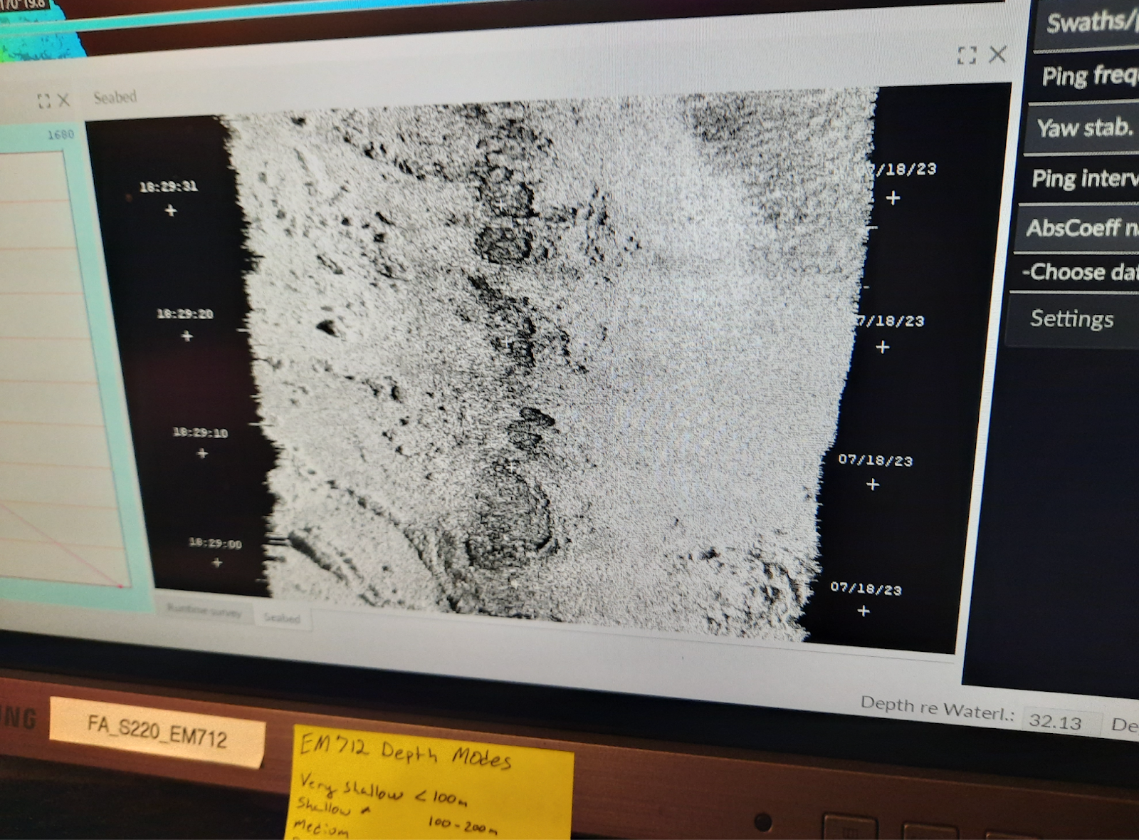
Backscatter is a visual representation of the surface of the seafloor.  Backscatter provides information about the intensity of the returned echos, from which the “hardness” of the bottom as well as other characteristics can be used to differentiate between different types of seafloor composition.  Darker colors represent harder surfaces such as rocks and hard coral and lighter colors represent softer surfaces such as sand and mud.  This information is important for ships to know for anchoring purposes, as well as benthic habitat characteristics.

The water column data shows us what is under the ship throughout the water column– from the surface of the water to the seafloor.  It detects bubbles, objects protruding from the seafloor, fish, or even a whale or a seal.

a triangular swath of echosounder data in different colors (red, green, blue) indicating the intensity of the returned echoes

Water column Data

photo of a computer screen displaying seafloor bathymetry (in black and white) from backscatter

Backscatter showing a representation of the seafloor

Finnegan and Elli sit in desk chairs in front of an array of computer monitors. There's a bookshelf filled with binders, an electrical box mounted to the wall, papers clipped to another wall. Finnegan and Elli are both wearing navy-colored NOAA logo-ed apparel.

TAS Elli Simonen with Survey Technician Finnegan Sougioultzoglou

Personal Log

Safety and Routine Checks

Before coming on board, I did not realize all the preemptive safety measures that need to be taken to ensure the health and safety of everyone on board.  The staff and crew need to be self-sustaining on all accounts; another person, equipment or supplies cannot be added mid-sail.  There are cooks onboard as well as medical staff.  There are 3 drills and situations that the entire crew participates in, including myself – Fire, Mariner Overboard and Abandon Ship.  You need to know the pattern of alarms for each, as well as where to go and what to do.  For example, for Mariner Overboard I go to the fantail of the ship, with others, and point at the person in the water until a small boat can go out and rescue them.  Each one of these drills is practiced periodically. Additionally there are two sets of rounds every hour, 24 hours a day – a deck round and engine rounds.  Deck rounds check all public spaces for anything abnormal.  Engine rounds check the engine room to see if everything is working properly.  Every week, refrigerators are checked for correct temperatures and water is checked for potential bacteria.

New Terms/Phrases

I’ve learned several acronyms and initials since I have been on board NOAA Ship Fairweather.  Sometimes I feel two consecutive sentences cannot be said without some type of abbreviation.  These are some that have become part of my vocabulary: 

  • HIC: Hydrographer in Charge
  • POD: Plan of the Day
  • SOP: Standard Operating Procedure
  • NM: Nautical Miles
  • CO: Commanding Officer

Jill Bartolotta: Sounds of the Deep, June 5, 2019

NOAA Teacher at Sea

Jill Bartolotta

Aboard NOAA Ship Okeanos Explorer

May 30 – June 14, 2019

Mission:  Mapping/Exploring the U.S. Southeastern Continental Margin and Blake Plateau

Geographic Area of Cruise: U.S. Southeastern Continental Margin, Blake Plateau

Date: June 5, 2019

Weather Data:

Latitude: 29°01.5’ N

Longitude: 079°16.0’ W

Wave Height: 2 feet

Wind Speed: 10 knots

Wind Direction: 128

Visibility: 10 nm

Air Temperature: 27.7°C

Barometric Pressure: 1021.3

Sky: few

Science and Technology Log

What is sonar?

Sonar is the use of sound to describe the marine environment. Sonar can be compared to satellites that use light to provide information about Earth, but instead of light, sound is used. It is used to develop nautical charts, detect hazards under the water, find shipwrecks, learn about characteristics of the water column such as biomass, and map the ocean floor. There are two types of sonar, active and passive. Active sonar is sonar that sends out its own sound wave. The sonar sends a sound wave (ping) out into the water and then waits for the sound to return. The return sound signal is called an echo. By assessing the time, angle, and strength of the return sound wave or echo one can learn many details about the marine environment. Passive sonar does not actively send out a sound ping, but rather listens for the sound from other objects or organisms in the water. These objects may be other vessels and these organisms may be whales or marine ecosystems such as coral reefs.

Sound waves move through the water at different speeds. These speeds are known as frequencies and the unit of measurement for sound is a hertz (Hz). Lower frequencies (example 18 kHz) are able to go farther down because they move slower and have more power behind them. It is like when a car goes down your street, pumping the bass (always seems to happen when I am trying to sleep) and you can hear it for a long time. That is because it is a low frequency and has longer wave lengths. Higher frequencies (example 200 kHz) move faster, but have less power. The sound waves should reach the bottom, an object, or biomass in the water column, but there may be no return or echo. High frequency sound waves are closer together. High frequencies give you a good image of what is happening near the surface of the water column and low frequencies give you a good idea of what is happening near, on, or under the ocean floor.

Type of Sonar on Okeanos Explorer

There are many types of sonar and other equipment aboard Okeanos Explorer for use during mapping operations. All have different capabilities and purposes. Together they provide a complete sound image of what is happening below us.

Kongsberg EM302 Multibeam Sonar

Multibeam sonar sends sound out into the water in a fan pattern below the hull (bottom) of the ship. It is able to map broad areas of the water column and seafloor from depths of 10 meters to 7,000 meters. Only the deepest trenches are out of its reach. It is the most appropriate sonar system to map seafloor features such as canyons and seamounts. The fan like beam it emits is 3-5.5x the water depth with a max swath range of 8 km. However, when you get to its depths below 5,000 meters the quality of the sound return is poor so scientists keep the swath range narrower to provide a higher quality of data return. The widest swath area scientists can use while maintaining quality is a depth of 3,300-5,000 meters. The user interface uses a color gradient to show you seafloor features (red=shallow and purple=deep).

Swath ranges for the multibeam sona
Swath ranges for the multibeam sonar at various depths. The y-axis shows the water depth in meters and the x-axis shows the swath width in meters. Photo credit: SST Charlie Wilkins, NOAA Ship Okeanos Explorer
Multibeam Sonar information
Some of the information that is collected using the multibeam sonar with labels describing their purpose. Photo Credit: NOAA OER

Backscatter

Backscatter uses the same pings from the multibeam. People use backscatter to model or predict physical or biological properties and composition of the sea floor. The coloring typically is in grayscale. A stronger echo looks brighter in the image. A weaker echo looks darker in the image. It gives you a birds-eye view of seafloor characteristics such as substrate density and seafloor features.

Backscatter and Bathymetry
Top image is backscatter showing you a birds-eye view of the ocean floor. The bottom image shows you what it looks like when backscatter is overlaid over the bathymetry layer. You are able to see intensity of the sound return, but floor features are more noticeable. Photo credit: NOAA OER

XBT

An Expendable Bathy-Thermograph (XBT) provides you with information on the temperature gradients within the water. When the temperature profile is applied to a salinity profile (taken from World Ocean Atlas) you are able to determine sound velocity or the rate at which the sound waves can travel through the water. When sound moves through water it does not move in a straight line. Its path is affected by density which is determined by water type (freshwater or saltwater) and temperature. Freshwater is less dense than saltwater and cold water is denser than warm water. The XBT information accounts for sound refraction (bending) through various water densities. When near shore XBTs are launched more frequently because the freshwater inputs from land alter density of the water and temperatures in the water column are more varied. XBTs are launched less frequently when farther from shore since freshwater inputs are reduced or nonexistent and the water column temperature is more stable. However, ocean currents such as the Gulf Stream (affecting us on this cruise) can affect density as well. The Gulf Stream brings warm water from the Gulf of Mexico around the tip of Florida and along the eastern coast of the United States. Therefore, one must also take into account which ocean currents are present in the region when determining the launch schedule of XBTs.

Loading the XBT Launcher
Senior Survey Technician Charlie Wilkins and Explorer in Training, Jahnelle Howe, loading the XBT launcher. XBTs are launched off the stern of the ship.
XBT Capture
Sound speed or velocity is determined by the density of the water, which is determined by temperature and salinity. Focus on the blue line in each graph. The first graph takes the information from the temperature and salinity graphs to determine sound speed. If we look at the first graph, we see that sound speed slows with depth. Sound speed slows because according to the second graph the temperature is colder making the water denser, thus affecting sound speed. Salinity does not vary much according to the third graph so its effect on density is most likely limited. Photo credit: NOAA OER

Simrad EK60 and EK80 Split-beam Sonar

Split-beam sonar sends out sound in single beam of sound (not a fan like the multibeam). Each transducer sends out its own frequency (example 18 kHz, 38 kHz, 70 KHz, 120 kHz, and 200 kHz). Some frequencies are run at the same time during mapping operations. Mapping operations typically do not use the 38 kHz frequency since it interferes with the multibeam sonar. Data collected with the use of the EK60 or EK80 provides information about the water column such as gaseous seeps, schools of fish, and other types of dense organism communities such as zooplankton. If you remember my “did you know” from the second blog, I discussed how sonar can be used to show the vertical diurnal migration of organisms. Well the EK60 or EK80 is the equipment that allows us to see these biological water column communities and their movements.

Water column information
Water column information collected with the EK60 or EK80 split beam sonar. If you look at the first row you can see, in the image to the left, the blue dots are at the top and in the second image the blue dots are moving back down into the water column as the sun rises. The process of organisms’ movement in the water column at night to feed is known as vertical diurnal migration. Photo Credit: NOAA OER

Knudsen 3260 Sub-bottom Profiler

The purpose of using a sub-bottom profiler is to learn more about the layers (up to 80 meters) below the ocean floor. It works in conjunction with the sonar mapping the ocean floor to provide more information about the bottom substrate, such as sediment type and topography features. Sub-bottom data is used by geologists to better understand the top layers of the ocean floor. A very low frequency is used (3.5 kHz) because it needs to penetrate the ocean sediment. It will give you a cross section of the sea floor so floor features can be detected.

Cross section of the ocean seafloor
Cross section of the ocean seafloor shows you substrate characteristics. Photo Credit: NOAA OER

Telepresence

Telepresence aboard the ship allows the science team to get mapping products and raw data to land on a daily basis. The science team can also live feed data collection to shore in real time. By allowing a land based shore team to see the data in real time you are adding another system of checks and balances. It is one more set of eyes to make sure the data being collected looks correct and there are no issues. It also allows a more collaborative approach to mapping, since you are able to involve a worldwide audience in the mission. Public viewers can tune in as well.  Support for the technology needed to allow telepresence capabilities comes in partnership with the Global Foundation of Ocean Exploration (GFOE). With GFOE’s help, the protocols, high-speed satellite networks, Internet services, web and social media interfaces, and many other tools are accessible when out to sea. The NOAA Office of Exploration and Research (OER) provides the experts needed to develop, maintain, and operate the telepresence systems while at sea, but also at shore through the Exploration Command Centers (ECCs) and the University of Rhode Island’s Inner Space Center.

Live interaction
Live interaction with Okeanos Explorer, Inner Space Center at URI/GSO, and a group of high school students. Photo credit: NOAA OER

All in all, the equipment aboard Okeanos Explorer is impressive in its abilities to provide the science team with a high quality and accurate depiction of the ocean floor and water column. The science team aboard is able to interpret the data, clean out unwanted data points, store massive data files on computers, and send it back to land daily, all while rocking away at sea. Very impressive and very cool!

Personal Log

I learned all about memes today. Apparently they are very popular on the ship. So popular, we are even in the middle of a meme contest. For those of you unfamiliar to memes like I was, a meme is a funny picture with a clever caption that makes you laugh or relates to something in your life. After my tutorial in meme making, we had a great time out on the bow of the ship playing corn hole and hanging out. The night was beautiful. The humidity subsided and there was a great breeze. After the sun set, I watched the stars come out and then went inside to learn more about the mapping process. I am starting to get a better understanding of what the science team is doing. You know the how and the why of it all. After I couldn’t keep my eyes open any longer, I made my nightly venture out onto the bow to look from some bioluminescence, the glittering of zooplankton in the night. A magical site. I will leave you wondering how the ocean glitters until one of my future blogs when I describe the process of bioluminescence.

Corn hole
General Vessel Assistant Sidney Dunn (left) and General Vessel Assistant Christian Lebron (right) playing corn hole on the bow at sunset.

Did You Know?

The SOFAR (Sound Fixing and Ranging) channel occurs in the world’s oceans between depths of 800 to 1000 meters in the water column. Because of the density and pressure around this channel, sound waves travel for an extended distance. It is thought that fin whales travel to this channel to communicate with other fin whales many kilometers away.

Helen Haskell: Bottom Sampling! June 17, 2017

NOAA Teacher at Sea

Helen Haskell

Aboard NOAA Ship Fairweather

June 5 – 26, 2017


Mission: Hydrographic Survey

Geographic Area of Cruise: Southeast Alaska – West Prince of Wales Island

Date: June 17, 2017

Weather Data (on day of bottom sampling –June 14th)

Wind:  27 knots from the west (110° true)

Visibility: 10 nautical miles

Barometer:  1005.3 hPa

Air temperature: 9.4°C

Cloud: 100% cover, 1000’

Location

54°54.4’N  132°52.3’W


Science and Technology Log 

IMG_2004
Hollings Scholar Carly LaRoche, TAS Helen Haskell, and LT Damian Manda with a bottom sample.

If you have ever taken a look at a nautical map, other than just depths listed on it, there will be symbols and definitions that provide information to help with safety and knowledge of the area.  For example, asterix-like symbols represent rocks, and a branch-like symbol represents kelp. Also written on the maps is information about the seafloor and what it is composed of, such as gravel, sand, or bedrock.  Here in southeast Alaska, off the coast of Prince of Wales Island, much of the data that is currently on the charts was collected over 100 years ago.  Fairweather’s mission is to collect new information to allow these charts to be updated, and this includes information on the seafloor too.

The other day I was tasked with joining a survey crew to conduct bottom sampling.  The assigned bottom sample locations are provided by the Operations branch at headquarters. The sheet managers adapt the locations if they think there are better locations that will provide information for anchoring or to help characterize different regions in the area.  With less than glassy water conditions on a windy and rainy day, the boats were launched and we moved to our first sample area.

IMG_0252
A bottom sampler

The technology behind sampling is a little more antiquated than other parts of the research I’ve seen. It involves hooking up a self-closing scoop like device to a rope, and lowering it in to the water until it hits the seafloor.  Ideally, the trigger is released when it hits the seafloor and it closes. With closed scoops, the bottom sampler is winched up, ideally full of whatever material is located on the seafloor in that immediate location.  There were three different styles of these bottom samplers and we quickly had a firm favorite that seemed to work the best.  Easing the boat in the swell to the location, the coxswains, Dennis and Denek, would keep the boat in position so we did not tangle the rope in the motor.  We could tell from the rope going slack when the bottom sampler had hit the sea floor, and a mechanical winch made the return journey easy.


Dumping the contents in to a bucket we were able to see the diversity of the seafloor in just a few samples.  Occasionally rocks or shells would get stuck in the mechanism and we’d have to repeat the procedure, but overall we had tremendous success.

IMG_1863
Carly, Denek, the coxswain and me getting some respite from the rain

There are international protocols to follow in collecting bottom samples. These allow for communication and consistency of data on navigational charts.  In general, the main medium of the sample is described, such as sand, mud or pebbles, and an adjective used to describe it, such as broken, sticky or soft. Color is also assigned to the sample as well as appropriate size of the grains (fine, medium or coarse).  Symbols are used for all this data: For example, ‘the sample is mostly fine brown sand with mud and a little bit of broken shell’ would be written fne br S M brk Sh.  Protocols indicate that if sampling is attempted three times in one location and it doesn’t work then ‘unknown’ is documented in that location.

IMG_1926
Success in our sampling

At each of the sampling locations, we marked the spot on the chart and took latitude and longitude coordinates. We also documented additional observations we had about the sample, including findings that were not included as data choices. For example, in our second sampling site we found what we thought initially were mammal hairs.   Several sites later we struck ‘gold’ again, finding what appeared to be more hairs in a mud matrix. Upon reflection and discussion, it’s possible they are more likely decomposing kelp fibers.  It would be interesting to have the samples analyzed to identify what these fibers/hairs come from.   We also found whole clamshells as well as having a sample that only contained water. Our thoughts with the water only samples were that perhaps we were hitting bedrock rather than failing on obtaining any kind of sediments.  We also observed that in the more sheltered bays, the samples were very odiferous dark mud. In both of these occasions, the landscape surrounding the bay was heavily logged, and it would be interesting to see if there were correlations between the logging and the dark sediments, perhaps containing higher levels of carbon material washed in from terrestrial sources. In one of these areas, documentation from 100 years ago suggested that at that time, the seafloor was gravel.


Personal Log

The bottom-sampling day was challenging day weather wise, both for the coxswains and the science crew, but very rewarding.  Due to the rough seas it wasn’t a good day to collect sonar data, and on days like this, other parts of the total data collection are put in to place.  Part of our work that day was to also do crosslines (sonar data verification) but the water conditions were too hazardous in certain directions of travel, and so it was decided that we should focus on bottom samples.   To be frank, this was my favorite day as a Teacher At Sea so far. Truth be told, I was reminded that I quite enjoy sticking my hand in a bucket of mystery ‘goop’ and trying to figure out what it is composed of.  The diversity of samples was completely surprising and finding hair samples, twice, completely intriguing.  It was great also to observe upcoming OPS officer, LT Damian Manda at work logging the data, and realize again, the role technological knowledge plays a role in the success of this research. And, thank you to Coxswain Dennis Brooks for taking most of the photos for this blog entry.


IMG_2047
Me and Carly at the end of the day


Word of the day:

Hollings Scholarship Program: this NOAA program provides undergraduate students with a ten week internship at a NOAA facility and academic assistance, as well as an orientation and symposium. For more information: http://www.noaa.gov/office-education/hollings-scholarship

Fact of the day:

Backscatter is the intensity of acoustic energy received by the sonar after interacting with the seafloor. Backscatter data can be used to help determine the surface of the seafloor.  In softer areas, perhaps a surface of mud, returns a weaker signal, but a harder surface, such as bedrock returns a stronger signal.  Hollings scholar Carly LaRoche from American University is on the boat for several legs this summer and is collecting and analyzing backscatter data in the area. Bottom sampling of the area is allowing Carly to compare the backscatter data with the sediments collected to see if there are correlations.

What is this?

IMG_0270

(Answer from previous blog: part of the vertical struts of an old pier at a former salmon canning factory.)

Acronym of the day: Used in bottom sampling

NATSUR:  Nature of surface  -example: mud, gravel, coral

NATQUA: Qualifying terms for NATSUR -example: sticky, soft, calcareous