
NOAA Teacher at Sea
Denise Harrington
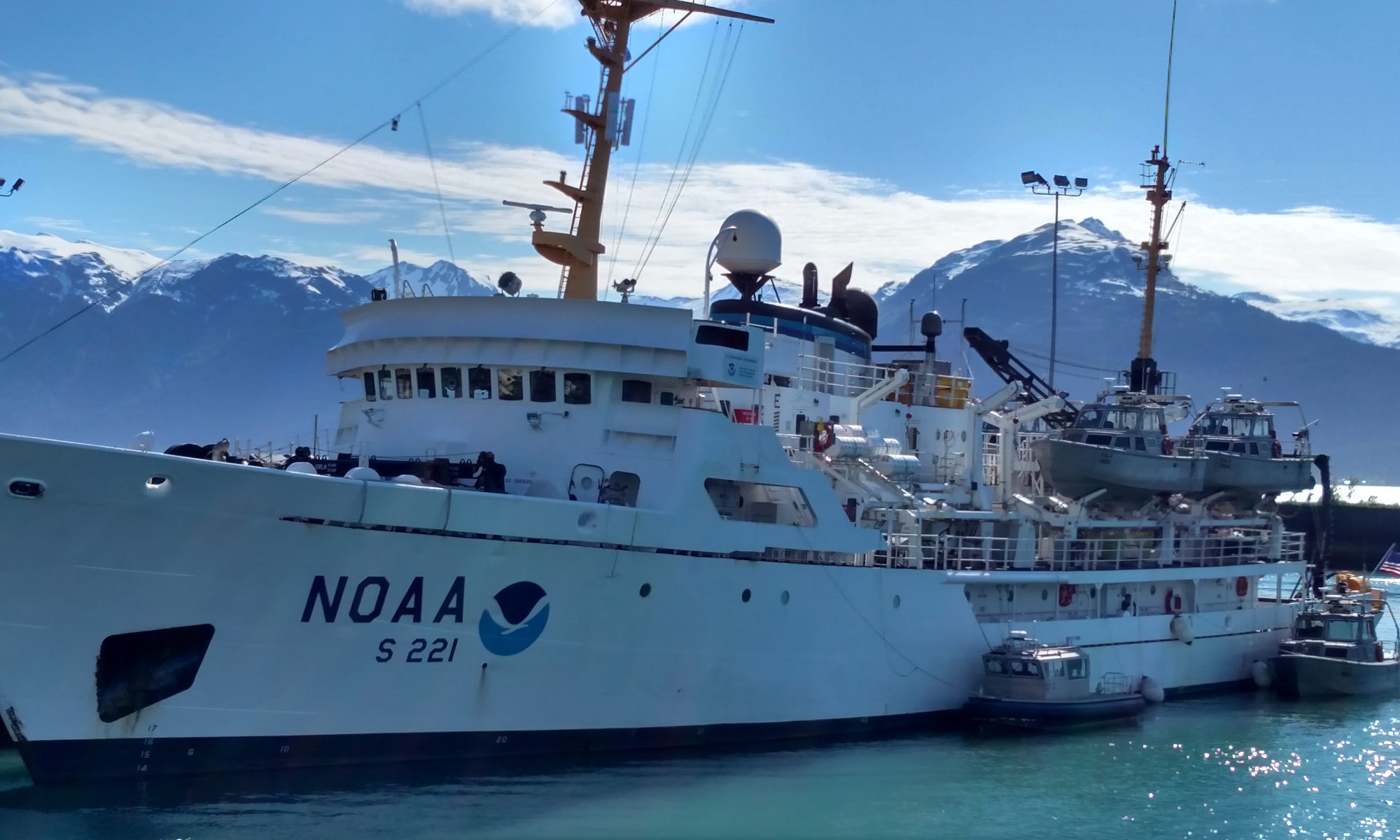
Aboard NOAA Ship Rainier
April 20 – May 3, 2014
Geographical Area of Cruise: North Kodiak Island
Date: May 2, 2014, 23:18
Location: 57o 43.041’ N 127o 152.32.388’ W
Weather from the Bridge: 13.09o C (dry bulb), Wind 1 knots @ 95o, clear, 0′ swell, balmy “crazy nice weather” say Able Seaman Jeff Mays
Our current location and weather can also be seen at NOAA Shiptracker: http://shiptracker.noaa.gov/Home/Map
Science and Technology Log
Today’s blog is all about post processing, or “cleaning up” the data and being on night shift. It is a balmy, sliver moon night at port here, in Kodiak. We have come a long way in the last two weeks, during which survey crews have been working hard to finalize a Cold Bay report from last season before they devote themselves entirely to North Kodiak Island. I am in the plot room with Lieutenant Junior Grade Dan Smith who is on Bridge Duty from midnight until 4 a.m. with Anthony Wright, Able Seaman.

People work around the clock on Rainier whether it be bridge watch, processing data, or in the engine room. One thing that makes the night shift a little easier is that there is no shortage of daylight hours in Alaska: within two months, there will be less than an hour of complete darkness at night.

In previous blogs, I described how the team plans a survey, collects and processes data. In this blog, I will explain what we do with the data once it has been processed in the field. Tonight, Lieutenant Dan Smith is reviewing data collected in Sheet 5, of the Cold Bay region on the South Alaskan Peninsula. In September, 2013, the team surveyed this large, shallow and therefore difficult to survey area. The weather also made surveying difficult. Despite the challenges, the team finished collecting data for Sheet 5 and are now processing all the data they collected.

While I find editing to be one of the most challenging steps in the writing process, it is also the most rewarding. Through the editing process, particularly if you have a team, work becomes polished, reliable and usable. The Rainier crew reviews their work for accuracy as a team and while Sheet 5 belongs to Brandy Geiger, every crew member has played a part in making the Sheet 5 Final Report a reality, almost. On the left screen, Lieutenant Smith is looking at one line of data. Each color represents a boat, and each dot represents the data from one boat, and each dot represents a depth measurement computed by the sonar. The right screen shows which areas of the map he has already reviewed in green and the areas he still needs to review in magenta.

While the plot room is calm today in Kodiak, there have been times when work conditions are challenging, at best.
.The crew continues on, despite the weather, so long as work conditions are safe.
Several days ago, Lieutenant Smith taught me the difference between a sonar ping that truly measured depth, and other dots that were not true representations of the ocean floor. Once you get an eye for it, you kill the noise quickly. In addition, when Lieutenant Smith finds a notable rise in the ocean floor he will “designate as a sounding.” Soundings are those black numbers on a nautical chart that tell you how deep the water is.

If the line has dots that rise up in a natural way, the computer program recognizes that these pings didn’t go as far down as the others and makes a rise in the ocean floor indicated with the blue line. It is the hydrographer’s job to review the computer processed data. One of the differences between a map and a nautical chart is the high level of precision and review to ensure that a nautical chart is accurate.


NOAA has several interesting online resources with more information about the differences between charts and maps: http://oceanservice.noaa.gov/facts/chart_map.html .
Now let’s kill some noise on this calm May evening.
In this image of a shipwreck on the ocean floor most sonar pings reached the ocean floor or the shipwreck and bounced soundings back to the survey boat. Look carefully, however, and you see white dots, representing pings that did not make it down to the ocean floor. Many things can cause these false soundings. In this case, I predict that the pings bounced back off of a school of fish. Here, the surveyor kills the “noise” or white pings by circling them with the mouse on his computer. It wouldn’t be natural for the ocean floor or other feature to float unconnected to the ocean floor, and thus, we know those dots are “noise” and not measurements of the ocean floor.
Lieutenant Smith estimates that at least half of his survey time is spent in the plot room planning or processing data. The window of time the team has in the field to collect data is limited by weather and other conditions, so they must work fast. Afterward, they spend long, but rewarding hours analyzing the data they have collected to ensure its accuracy and to provide synthesized information to put into a nautical chart that is easy to use and dependable. Lieutenant Smith believes that in many scientific careers, as much time or more time is spent planning, processing and analyzing data than is spent collecting data.
Personal Log
As we post process our data, I too, begin post processing this amazing adventure. I am hesitant to leave: I have learned so much in these two short weeks, I want to stay and keep learning. But at NOAA we all have many duties, and my collateral, wait–my primary duty is to my students and so, I must return to the classroom. I will leave many fond memories and a camera, floating somewhere in Driver Bay, behind me. I will take with me all that I have learned about the complexity of the ocean planet we live on and share my thirst to know more back to the classroom where we can continue our work. I will miss the places I’ve seen and the people I met but look forward to the road or channel of discovery that awaits me and my students.

Did You Know? The Sunflower Sea Star is the largest and fastest moving sea star travelling up to one meter per minute.

Below are a few photo favorites of my time at sea.


